Abstract
Pass@ is widely used to report the reasoning performance of LLMs, but it often produces unstable and potentially misleading rankings, especially when the number of trials (samples) is limited and computational resources are constrained. We present a principled Bayesian evaluation framework that replaces Pass@ and average accuracy over trials (avg@) with posterior estimates of a model's underlying success probability and credible intervals, yielding stable rankings and a transparent decision rule for differences. Evaluation outcomes are modeled as categorical (not just 0/1) with a Dirichlet prior, giving closed-form expressions for the posterior mean and uncertainty of any weighted rubric and enabling the use of prior evidence when appropriate. Theoretically, under a uniform prior, the Bayesian posterior mean is order-equivalent to average accuracy (Pass@), explaining its empirical robustness while adding principled uncertainty. Empirically, in simulations with known ground-truth success rates and on AIME'24/'25, HMMT'25, and BrUMO'25, the posterior-based procedure achieves faster convergence and greater rank stability than Pass@ and recent variants, enabling reliable comparisons at far smaller sample counts. The framework clarifies when observed gaps are statistically meaningful (non-overlapping credible intervals) versus noise, and it naturally extends to graded, rubric-based evaluations. Together, these results recommend replacing Pass@ for LLM evaluation and ranking with a posterior-based, compute-efficient protocol that unifies binary and non-binary evaluation while making uncertainty explicit. Source code is available at GitHub .
Introduction
Large language models (LLMs) have moved rapidly from research artifacts to everyday infrastructure [1, 2]. Students use them for homework and exam preparation; developers rely on them for code synthesis and refactoring [3]; analysts and clinicians use them for decision support; and agents built atop LLMs are increasingly embedded in workflows across industry and government. This demand has catalyzed unprecedented investment: specialized chips, datacenters, and startups dedicated to LLM training, serving, and tooling [4]. As deployment accelerates, trust, oversight, and comparability become central: how we evaluate LLMs directly shapes which models are adopted, what progress is declared, and how resources are allocated [5, 6, 7, 8, 9, 10, 11].
Evaluation, however, remains the weakest link in the LLM pipeline. Alongside advances in model efficiency and compression[12, 13, 14, 15, 16, 17, 18, 19], training and fine-tuning methods such as parameter-efficient fine-tuning (PEFT), low-rank adaptation (LoRA), and reinforcement learning from human feedback (RLHF) [20, 21, 11], and inference/decoding (sampling strategies, caching, efficient attention) [22, 23], the community still leans on simple, yet flawed, success rates and Pass@-style metrics to summarize capabilities [24]. These practices are convenient but fragile. On small or costly benchmarks (e.g., math reasoning sets with only tens of problems such as AIME) [25, 26], Pass@ or single-run accuracy often produce unstable rankings [27], are sensitive to decoding choices and seed effects [22, 28], and provide little guidance on whether observed gaps are meaningful or mere noise [29, 30]. Averaging across multiple runs ("avg@") helps but is compute-hungry [31], offers no unified way to handle graded/rubric outcomes, and lacks a principled decision rule for significance [29, 32, 33].
This paper takes a different approach: we treat evaluation itself as a statistical inference problem. We introduce a posterior-based framework that replaces Pass@ and avg@ with estimates of a model’s underlying success probabilities and associated uncertainty [34]. Outcomes are modeled as categorical [35] rather than purely binary: each item can yield correct, partially correct, formatting-error, refusal, or rubric-defined levels. A Dirichlet prior over these categories yields closed-form posterior means and credible intervals for any weighted rubric, allowing the evaluator to report both a point estimate and principled uncertainty with negligible overhead. In the binary special case under a uniform prior, its posterior mean is order-equivalent to average accuracy, explaining the empirical robustness of avg@ while making uncertainty explicit.
The framework addresses four persistent pain points. 202 Convergence: as shown in Figure 1, we ideally want methods that can converge to the true underlying ranking with the smallest number of trials, but different approaches can have significantly different convergence speeds. 203 Credible intervals: a simple, transparent rule - do not declare a winner when intervals overlap - reduces leaderboard churn and over-interpretation of tiny gaps by introducing a compute-efficient credible interval (CI). Updates are analytic; one can monitor interval widths online, and allocate additional trials only when needed (no Monte Carlo/bootstrap simulations are required for CI estimation). 204 Categorical evaluation: our approach unifies binary and non-binary evaluation. Graded rubrics are natural in this framework, so one can evaluate step-by-step reasoning, partial credit, or judge categories without ad hoc aggregation. 205 Prior information: we can incorporate prior evidence when appropriate (e.g., reuse of stable rubric distributions across closely related tasks or versions).
We validate the approach in two settings: In controlled simulations with known ground-truth success rates, the posterior procedure converges to correct rankings with fewer samples than Pass@ and recent variants, and it flags when ties are statistically unresolved. On real math-reasoning benchmarks (AIME'24/'25 [25, 26], HMMT'25 [36], and BrUMO'25 [37]-derived sets), we observe the same pattern: the posterior method achieves greater rank stability at far smaller sample counts than Pass@, while clarifying when differences are meaningful versus noise. Practically, this yields a computationally efficient protocol that is easy to implement and audit.
We summarize our contributions as follows:
- A unified Bayesian evaluation framework. We model per-item outcomes as categorical with a Dirichlet prior, yielding closed-form posterior means and credible intervals for any weighted rubric, with binary evaluation as a special case. This unifies 0/1 and graded evaluations and supports reuse of prior evidence when justified.
- A compute-efficient, interval-aware protocol. We provide a simple recipe: report posterior means with credible intervals; only declare differences when intervals do not overlap; adaptively allocate additional samples until intervals meet pre-specified widths. This protocol naturally supports sequential/online evaluation.
- Empirical evidence on simulations and math benchmarks. On synthetic data with known ground truth and on AIME’24/’25, HMMT'25, and BrUMO'25 datasets, our method achieves faster convergence and greater rank stability than Pass@ and recent variants, enabling reliable comparisons with far fewer samples.
Bayesian Framework for Evaluating LLM Performance
Background: The Pass@ Metric and Its Limitations
Evaluation metrics for LLMs aim to quantify performance on tasks like reasoning or programming, but they often struggle to provide reliable relative rankings across models. Pass@, for instance, estimates the probability of at least one correct answer within model attempts (see Appendix 15 for details). While convenient, this metric exhibits high variance [38], particularly when approaches the total number of trials, , resulting in unstable rankings [24]. Small fluctuations in correctness can distort comparisons, particularly in benchmarks with few problems or limited computational resources, raising doubts about its suitability for differentiating model capabilities. If a metric cannot consistently distinguish stronger models from weaker ones, its value as a benchmarking tool is undermined [27].
Estimating uncertainty in Pass@ scores is also challenging, as it lacks closed-form expressions for variance, relying instead on computationally intensive approximations like bootstrapping. A truly effective metric should yield reliable performance rankings with a minimal number of trials, prioritizing both accuracy and efficiency in resource-constrained environments. To address these limitations, we propose a Bayesian evaluation framework that provides more stable estimates of performance, incorporates uncertainty, and facilitates robust relative comparisons across models [34, 39, 40].
Results Matrix
Consider a results matrix for an LLM evaluated on a test set comprising questions. Due to the stochastic nature of LLM sampling, responses may vary across independent trials, so we run the LLM times per question. The outcomes are captured in the matrix , where element represents the score in the th trial for the th question. This score is an integer ranging from to a maximum value , reflecting a rating system with categories. In the binary case (), 0 indicates an incorrect answer and 1 a correct one, though we accommodate more nuanced rubrics generally.
Weighted Performance Metric
For the th question, , there is an underlying probability that the LLM's answer falls in the th category. We denote as the -dimensional vector with elements , . If all were known, we could calculate a desired performance metric as a weighted average over these probabilities:
where is a -dimensional vector of constant weights. For example, if , then represents the average category label. In the case where , this average corresponds to the mean probability of a correct answer over the entire test set. However, we allow for a general choice of to accommodate a wide range of possible metrics.
Bayesian Estimator and Uncertainty for the Performance Metric
In principle, we could estimate by running an arbitrarily large number of trials with the LLM, yielding an accurate estimate of . However, we are typically constrained to small due to limited computational resources. Our goal is to develop a Bayesian approach to estimate and its associated uncertainty given a finite . The first step is to construct , the posterior probability of given the th row of the matrix , denoted . This posterior depends on the data in and a chosen prior distribution for the unknown underlying probability vector . The prior could be uniform (assuming no prior information) or incorporate previously gathered evidence about the LLM's performance. The Bayesian framework focuses on two quantities: the first is the mean of over the joint posterior for all questions, which we denote as . This is a Bayesian optimal estimator, minimizing the quadratic loss function over all possible estimators , where the expectation value is over all possible and realizations of [41]. The second quantity is the variance , which quantifies the uncertainty of the estimate. Both and have exact closed-form expressions, derived in Appendix 10, and can be simply calculated for any using Algorithm 1.
Function EvaluatePerformance$R$, $[R^0]$, $w$
State input: $M N$ matrix $R$ of results, with each element $R_ i = 0,,C$
State $$ weight vector $w = (w_0,,w_C)$ defining performance metric $\pi$
State optional input: $M D$ matrix $R^0$ of results for prior; otherwise $D=0$
State output: performance metric estimate $$ and associated uncertainty $$
State $T = 1+C+D+N$
For $ = 1$ to $M$ // Tally results in $R$ and $R^0$
For $k = 0$ to $C$
State $n_ k = _i=1^N _k,R_ i$
State $n^0_ k = 1+_i=1^D _k,R^0_ i$
State $_ k = n^0_ k + n_ k$
EndFor
EndFor
State $ = w_0 + 1M T _=1^M _j=0^C _ j(w_j - w_0)$
State $ = ^1/2$
State return $$, $$
EndFunction
Using Uncertainty Estimates to Decide Significance of Performance Differences
In general, the expressions for and are valid for any and , and do not rely on asymptotic arguments like the central limit theorem (CLT). However, there are useful simplifications that occur in specific limiting cases. For example as the size of the test set becomes large, we can derive not just the moments of the posterior distribution for , but also its shape, which becomes approximately Gaussian: . This allows us to assess whether two methods exhibit a statistically significant performance difference. Consider results matrices and from two approaches, with corresponding means , and standard deviations , . The distribution of the performance difference is a convolution of the individual posteriors, yielding another normal distribution: , where the mean of the difference is , and the standard deviation is . To determine our confidence in the ranking of the two methods, we need to determine the probability that . This can be done by calculating the absolute -score, . The probability that the ranking based on and is correct (the ranking confidence ) is given by . For example corresponds to .
Equivalence of Bayesian and Average Rankings for Uniform Prior
In the results below, we will denote ranking based on the Bayesian estimator with a uniform prior as Bayes@. Because is related to a naive weighted average accuracy via a positive affine transformation, it turns out the ranking based on the average, denoted as avg@, is identical to Bayes@ (for the detailed proof, see Appendix 11). In the large-trial limit , the value of approaches the average, as expected, but the ranking equivalence holds at all finite . This relationship also extends to uncertainty quantification, where the standard deviation of the average relates to the Bayesian standard deviation by a scaling factor, providing a concrete method to compute uncertainty in the average without relying on the Central Limit Theorem. This is particularly advantageous in small-sample regimes common in LLM evaluations, where CLT-based methods often underestimate uncertainty and produce invalid intervals (e.g., extending beyond [0,1] or collapsing to zero) [42]. As highlighted by [42], Bayesian approaches with uniform priors (e.g., Beta(1,1) in the binary case) yield well-calibrated credible intervals even for datasets with fewer than a few hundred datapoints, outperforming CLT approximations in coverage and handling complex structures like clustered data.
Gold Standard for Ranking
Strictly speaking, the underlying true ranking of LLMs for a particular performance metric is unknown, because it would require determining the infinite trial limit, , for each LLM. In practice, we have to settle for an approximation to , calculated at some large but finite value (for example in our LLM experiments). Specifically, we use Bayes@ - which is the same as the ranking based on avg@- as our "gold standard" or reference ranking [43]. In other words, rankings using smaller will be compared to this gold standard to assess their accuracy.
For this comparison, we employ Kendall's , a nonparametric correlation coefficient that measures ordinal agreement between two rankings by comparing the number of concordant and discordant pairs of models. The coefficient ranges from (perfect inversion) to (perfect agreement), with indicating no association. We specifically use the variant, which properly accounts for ties in the rankings (e.g., the intentional tie in our simulation below), ensuring that equivalences do not artificially inflate the correlation. See Appendix 16.1.1 for further discussion and formal definitions.
To validate our claims about the gold standard as Bayes@, specifically to determine which evaluation methods converge to the true ranking, we conduct a simulation using biased coins as a metaphor for LLMs. In this setup, we already know the underlying performance distribution (the success probabilities for each question), allowing us to establish a known ground truth . We generate sets of these probabilities, with values of , representing different LLMs (note the tie at to test handling of equivalent performances). We run experiments for questions, where each LLM "answers" all the questions in each trial according to its success probabilities . Panel (a) of Figure 2 shows results without bootstrapping: we generate 1000 independent matrices, each with trials; for each step in the number of trials (from to ), we compute scores using Pass@ (, , and with an unbiased estimator Equation 21), Bayes@, Pass^ (Equation 22), G-Pass@ (Equation 23 with ), and mG-Pass@(Equation 24), then derive rankings and compare them to the gold standard using Kendall's as a measure of rank correlation (where indicates perfect alignment with the gold standard), and report the average over the matrices. Note that we do not explicitly show average accuracy avg@ because it is equivalent to Bayes@, as discussed in Section 2.6. In practice, we are computationally limited to a small number of trials per question. To examine what happens with only trials, we apply two methods of bootstrapping with replacement to the matrix, allowing us to estimate how results differ from the ideal case with a large number of independent matrices (panel a). For both methods, we generate bootstrap replicates for each of the to trials, derived from a single matrix. Panels (b) and (c) of Figure 2 illustrate this using two bootstrapping schemes. In the first scheme (panel b, column-wise bootstrapping), we resample trial indices; in the second (panel c, row-wise bootstrapping), we resample answers independently for each question. In both cases, the resulting bootstrap replicates are used to recompute evaluation scores, rankings, and values, which are then averaged to produce smoothed convergence curves. The two bootstrapping approaches yield nearly identical behavior, and both closely match the baseline in panel (a). This demonstrates that the convergence behavior is robust and not sensitive to the ordering of answers in either the rows or columns of . Though in our LLM mimic simulations, we do not have to use bootstrapping (since we can easily generate an arbitrarily large number of matrices), in actual LLM experiments, we have limited trial data, and these results show that bootstrapping provides a viable way of estimating statistical properties like convergence.
As seen in Figure 2, Bayes@ begins with relatively high agreement with the gold standard and converges much faster to than Pass@ and its variants, which suffer from greater variance and bias at small . All methods eventually converge to the same ranking, but their rates of convergence differ substantially. This makes the convergence rate a crucial factor when choosing between different LLM evaluation methods.
Potential benefits of non-uniform priors
While the convergence results in figure 2 demonstrate that Bayes@ with a uniform prior outperforms alternatives like Pass@ in ranking models, there are scenarios where non-uniform priors can achieve even faster convergence. This is the case when we have data from models that are related or closely correlated to the ones we are ultimately interested in ranking. Potential examples include: i) results from an older version of a model used as a prior for ranking a newer version; ii) a non-quantized version (where running trials is computationally expensive) used to provide prior data for a quantized version (where achieving large is cheaper); iii) a base model used to provide prior data for a fine-tuned one. Though a full exploration of these kinds of priors will be left to future work, in this section, we will show the potential benefits through our synthetic biased-coin LLM models, introduced in Sec. 2.7.
We start with a set of eight "original" models with , labeled by . Each model consists of a set of success probabilities drawn from a distribution Beta. We fix these probabilities for all the numerical experiments described below, and their averages for the eight models are: [0.3021, 0.3166, 0.4144, 0.4985, 0.5351, 0.5759, 0.6679, 0.7487]. Hence for the original models higher corresponds to higher overall accuracy. We now imagine an "update" of model that mimics some kind of revision, fine-tuning, or other modification. Because the performance of the updated model should be correlated with the original, we model the update as a stochastic perturbation to the Beta distribution from which success probabilities are drawn: for updated model the values are drawn from Beta, where and are random integers of unit magnitude. For the updated models the value of may not strictly increase with , so the ranking of models could be different than the original. Fig. 3(a) shows a histogram of the Kendall's values comparing the original model set (described above) and 50k possible updated sets drawn using this stochastic procedure. A value of 1 corresponds to exactly the same ranking, and we see that the mean over the 50k realizations is 0.88. Hence there is some correlation between the original and updated rankings, but in the vast majority of cases (about 86% of the updates), the ranking has changed for the updated models.
The question we would like to ask is whether we can use the results from the original models as priors to help speed up convergence when ranking the updated models. To employ a non-uniform prior for a given model, we follow the procedure described in Appendix 10, and incorporate the prior via the results matrix corresponding to trial results over questions using the original model. Combined with trial results from the updated model, we get the Bayes@ accuracy estimate for the updated model. These estimates are then used to rank the 8 updated models. Because we know the values for this set, we know the true ranking, and we can compare the estimated and true rankings via Kendall's .
For each choice of and we run 50k replicates, with each replicate consisting of a set of stochastic updates of the original models. The mean values over all these replicates are shown in Fig. 3(b) as a function of for several different . As expected, the curves increase with , since the ranking becomes more certain with more trials, but the convergence properties vary. The dashed line is the case of a uniform prior (), while the solid lines represent five different non-uniform prior scenarios, with , 2, 4, 8, and 16. For small and small we see a clear benefit of the non-uniform prior: already at , the value of starts higher than the uniform case, and remains so until the latter catches up for . Thus when we have prior data available, we can extract more accurate rankings with just a small number of trials of the updated model, relative to the uniform case. However there is a possibility to over-emphasize the prior: when and 16, the benefit for small turns into a disadvantage at larger . The curves dip beneath the result, indicating that the prior has impeded accurate ranking. Fig. 3(c) shows these trends more clearly by plotting , the difference between the for each and the uniform with . So we see that priors have to be used judiciously, with a large enough to nudge the ranking in the correct direction, but not too large to outweigh the results from the updated models. One of the goals of our future work will be to establish practical guidelines for in different real-world use cases.
Ranking with Uncertainty
In Section 2.5, we described how uncertainty estimates from the Bayesian approach can be used to evaluate the relative performance of two models. Here, we extend these ideas to incorporate uncertainty into the ranking of multiple models. We do this via our biased-coin LLM mimics, which we denote LLM for , described in the previous section. To incorporate a chosen credible interval in the ranking, we order their values from highest to lowest, choose the appropriate threshold (for example for 95% CI in the ranking), and assign two consecutive methods the same ranking if the absolute -score falls below this threshold.
The first row of Table 1 shows the underlying gold standard ranking for all the LLM mimics, since in this case we know the true values. Note the tie between LLM and LLM, because their is the same. The second row shows the Bayes@ ranking without a credible interval (CI) and the third row shows Bayes@ incorporating the CI. The Bayes@ ranking without CI aligns with the gold standard, except for two differences: the order of and is swapped, and the tie between and is not captured, which is expected since this ranking relies solely on estimates without accounting for uncertainty . In contrast, the third row, which incorporates the CI, reveals multiple ties across several models. Interestingly, and are now indistinguishable at the CI. Despite the fact that would be an atypically large number of trials for an actual LLM evaluation, it is insufficient to confidently distinguish the small performance difference ( vs. 0.6213) between the two models.
| LLM mimic | 0LLM | 0LLM | 0LLM | 0LLM | 0LLM | 0LLM | 0LLM | 0LLM | 0LLM | 0LLM | 0LLM |
|---|---|---|---|---|---|---|---|---|---|---|---|
| Gold Standard | 11 | 22 | 33 | 55 | 44 | 66 | 77 | 77 | 88 | 99 | 1010 |
| Bayes@ (w/o CI) | 11 | 33 | 22 | 55 | 44 | 66 | 77 | 88 | 99 | 1010 | 1111 |
| Bayes@ (w/ CI) | 11 | 22 | 22 | 33 | 33 | 44 | 55 | 55 | 55 | 66 | 77 |
To quantify the trials needed to reliably separate models with closely matched performance, we simulated the probability of correctly ranking above as a function of the number of trials , shown in the left panel of Figure 4. At , the probability of obtaining the correct ranking is . The right panel plots the absolute -score versus ; at , the , corresponding to approximately confidence (though the plots exhibit some noise due to simulation variability). These values closely align with the empirical probabilities in the left panels.
We also determined the minimum sample size needed to achieve z-scores of and , corresponding to CI of approximately and , respectively, for distinguishing between models. These thresholds occur at about and . At these values, the simulated probability of correctly ranking the models is and , respectively, which is closely consistent with expectations given the inherent noise in the results. These results underscore the computational cost of distinguishing models whose true performance metrics differ only slightly. In our biased-coin setup, the underlying success probabilities were and , yet reliably establishing this distinction requires nearly trials. Such large sample requirements highlight the importance of considering both uncertainty and convergence rates when interpreting ranking-based evaluations.
Experiments
In this section, we empirically validate our proposed evaluation methods using real-world datasets, focusing on ranking LLMs for mathematical reasoning tasks. We employ bootstrapping to compute the expected value of each evaluation score at a given . First, we present rankings of LLMs on the AIME'24, AIME'25, BrUMO'25, and HMMT'25 datasets without accounting for variance, based solely on evaluation scores (with ties occurring when scores are identical). Subsequently, we demonstrate how incorporating uncertainty in these scores can alter rankings across different datasets. Building on the discussion in Section 2.7, we adopt the ranking derived from avg@ (equivalently, Pass@ evaluated on the same 80 trials) or Bayes@ (uniform-prior Bayesian estimator) as our gold standard for comparing current LLMs, noting their equivalence in rankings (as proven in Section 2.6). For each from to (with Pass@ and similar methods starting from to avoid computation with insufficient samples), we compare the rankings produced by various evaluation methods against this gold standard, reporting the average Kendall's over bootstrapped resamples to estimate the expected rank correlation at each step (assuming independence among questions and trials).
Convergence to Gold Standard
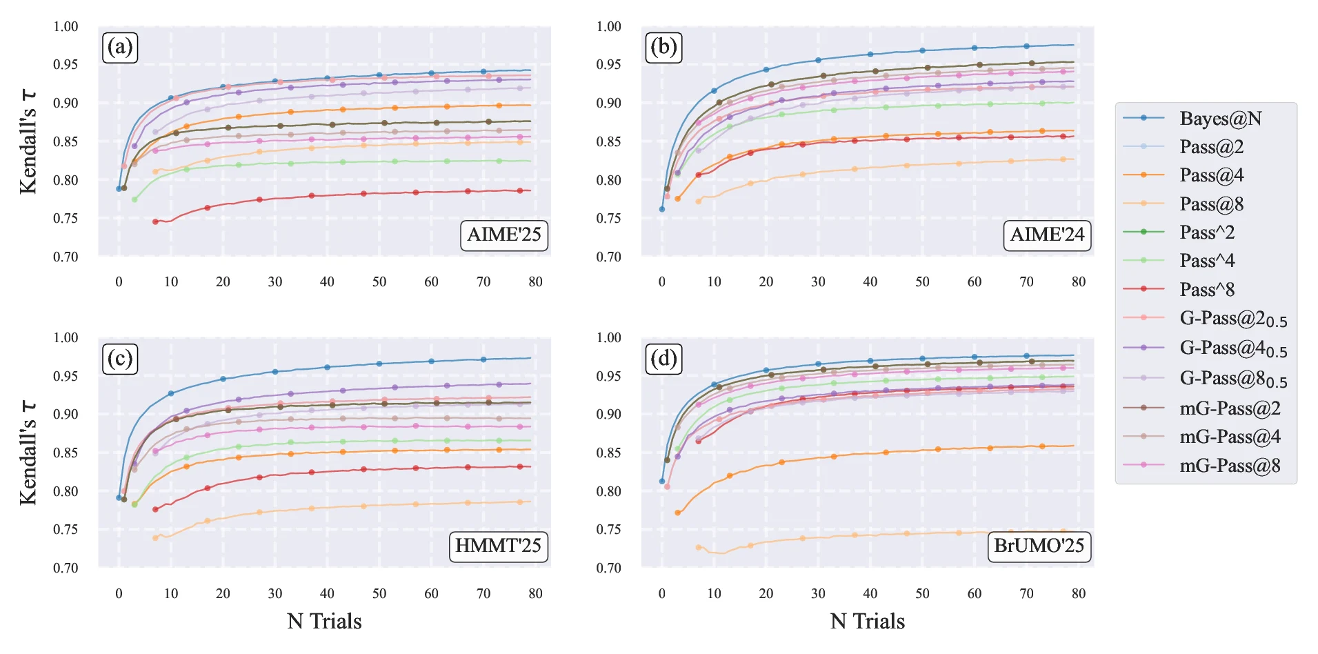
To assess the ability of different evaluation methods to compare the performance of different LLMs, we plot the average Kendall's against the gold standard as a function of the number of trials in Figure 5, combining results from AIME'25 (panel a), AIME'24 (panel b), HMMT'25 (panel c), and BrUMO'25 (panel d). Across all datasets, the Bayes@ and avg@ curves overlap completely (so we only plot Bayes@) and demonstrate the fastest convergence to high values, indicating robust alignment with the gold standard even in low-sample regimes. In all four datasets, Bayes@ reaches by and approaches at . The only exception is AIME'25, where is achieved by , but the curve converges to at .
In contrast, Pass@ variants () and their variations (e.g., Pass^, G-Pass@ with , mG-Pass@) start with lower Kendall's compared to Bayes@ and converge more slowly in all four datasets. At every , Bayes@ consistently shows faster convergence and higher agreement with the gold standard. These findings align with our biased-coin simulations in Section 2.7, demonstrating that the Bayesian method best satisfies the gold-standard criteria - low uncertainty, minimal ties, and rapid convergence - across diverse mathematical reasoning benchmarks.
Rankings With Credible Intervals
Following the methodology of Section 2.7.2, we compare model rankings across four datasets (AIME'25, AIME'24, HMMT'25, and BrUMO'25) using Bayes@ as the gold standard (see Figure 5). Table 2 summarizes these comparisons by reporting, for each dataset, two versions of the ranking: the rank with a CI and the rank without CI. The "w/ CI" rank accounts for uncertainty in the Bayes@ scores and therefore allows models with overlapping CIs to share the same rank; the "w/o CI" rank is the strict ordering determined by the point estimates of Bayes@ for that dataset.
Table 2 indicates that point-estimate rankings diverge from those accounting for credible intervals. Qwen Qwen3-30B-A3B-Thinking-2507 and Qwen Qwen3-4B-Thinking-2507 consistently secure the top positions across all four datasets; specifically, the dominance of the 30B model is statistically distinguishable at the CI level in every case. Conversely, the relative ordering of the remaining models varies by dataset.
When incorporating CIs, we observe that while all four datasets exhibit five tied groups, the extent of ambiguity varies significantly. AIME'25 yields the fewest distinct ranks (up to 11), followed by AIME'24 (up to 13), and both HMMT'25 and BrUMO'25 (up to 14). This compression of ranks indicates greater uncertainty in the Bayes@ gold standard for AIME'25 (due to more extensive ties) compared to the others under our current trial budget. Intuitively, this higher uncertainty in AIME'25's gold-standard scores implies that more additional trials would be required for that dataset to empirically produce a statistically stable ranking; conversely, we can be more confident in the estimated gold standards for AIME'24, HMMT'25, and BrUMO'25 given the current number of trials. This distinction also explains why AIME'25 reaches a Kendall’s of 0.95 at , whereas the other three datasets converge to at the same sample size in Figure 5.
| 2*Model | 2cAIME'25 | 2cAIME'24 | 2cHMMT'25 | 2cBrUMO'25 | ||||
|---|---|---|---|---|---|---|---|---|
| 0w/ CI | 0w/o CI | 0w/ CI | 0w/o CI | 0w/ CI | 0w/o CI | 0w/ CI | 0w/o CI | |
| Qwen Qwen3-30B-A3B-Thinking-2507 | 11 | 11 | 11 | 11 | 11 | 11 | 11 | 11 |
| Qwen Qwen3-4B-Thinking-2507 | 22 | 22 | 22 | 22 | 22 | 22 | 22 | 22 |
| gpt-oss gpt-oss-20b-high | 33 | 33 | 33 | 55 | 33 | 44 | 66 | 1111 |
| gpt-oss gpt-oss-20b-medium | 33 | 44 | 33 | 33 | 22 | 33 | 77 | 1212 |
| Microsoft Phi-4-reasoning-plus | 33 | 55 | 33 | 44 | 33 | 55 | 33 | 55 |
| NVIDIA AceReason-Nemotron-1.1-7B | 44 | 66 | 55 | 99 | 44 | 66 | 33 | 44 |
| Microsoft Phi-4-reasoning | 55 | 77 | 55 | 1010 | 55 | 88 | 44 | 77 |
| gpt-oss gpt-oss-20b-low | 55 | 88 | 66 | 1212 | 1111 | 1717 | 1111 | 1717 |
| OpenThinker OpenThinker2-32B | 55 | 99 | 44 | 88 | 55 | 77 | 22 | 33 |
| Light-R1 Light-R1-14B-DS | 55 | 1010 | 44 | 66 | 66 | 1111 | 44 | 88 |
| FuseO1 FuseO1-DeepSeekR1-QwQ-SkyT1-Flash-32B | 55 | 1111 | 44 | 77 | 66 | 99 | 33 | 66 |
| NVIDIA NVIDIA-Nemotron-Nano-9B-v2 | 66 | 1212 | 66 | 1111 | 66 | 1010 | 55 | 1010 |
| LIMO LIMO-v2 | 66 | 1313 | 77 | 1313 | 77 | 1212 | 55 | 99 |
| EXAONE EXAONE-4.0-1.2B | 77 | 1414 | 88 | 1414 | 77 | 1313 | 1010 | 1515 |
| OpenR1 OpenR1-Distill-7B | 77 | 1515 | 99 | 1515 | 1010 | 1616 | 88 | 1313 |
| OpenThinker OpenThinker3-1.5B | 88 | 1616 | 1010 | 1616 | 88 | 1414 | 99 | 1414 |
| NVIDIA OpenReasoning-Nemotron-1.5B | 88 | 1717 | 1111 | 1717 | 99 | 1515 | 1010 | 1616 |
| DeepSeek DeepSeek-R1-Distill-Qwen-1.5B | 99 | 1818 | 1212 | 1919 | 1212 | 1818 | 1313 | 1919 |
| Sky-T1-32B-Flash Sky-T1-32B-Flash | 1010 | 1919 | 1212 | 1818 | 1313 | 1919 | 1212 | 1818 |
| Bespoke-Stratos Bespoke-Stratos-7B | 1111 | 2020 | 1313 | 2020 | 1414 | 2020 | 1414 | 2020 |
Convergence
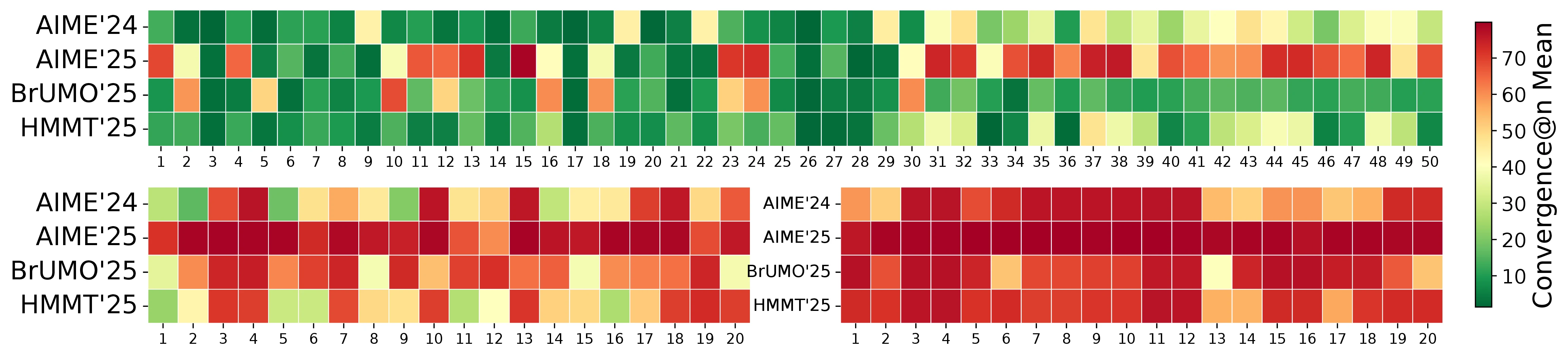
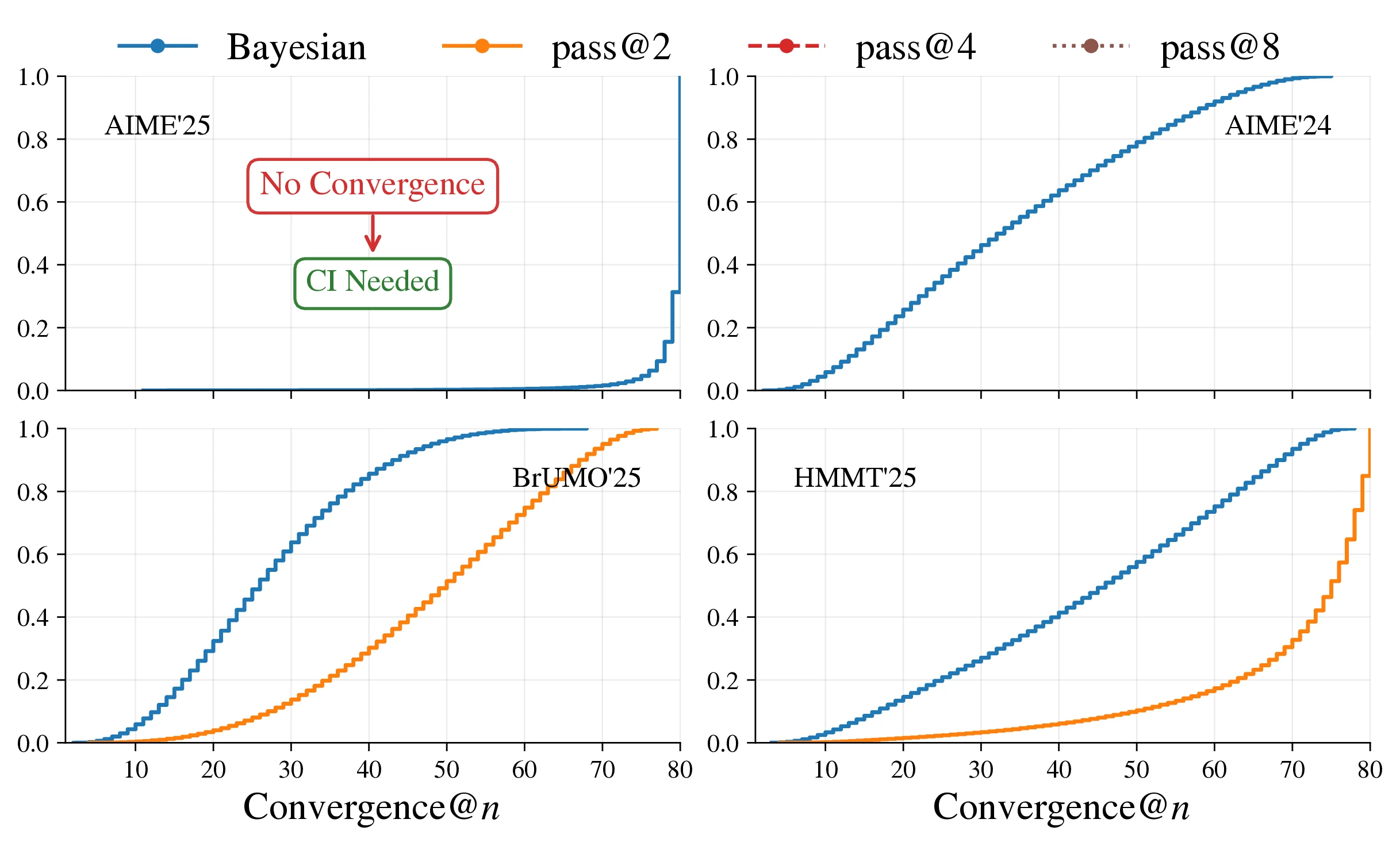
In this section, we investigate the convergence of model rankings, building on the showcase figure (Figure 1). We define convergence@ as the smallest trial at which the ranking induced by the first trials matches the gold standard ranking from all 80 trials (without bootstrapping) and remains unchanged thereafter.
Lower convergence@ values indicate that fewer trials are sufficient to achieve stable rankings. As detailed in the caption of Figure 1, the figure displays the probability mass functions (PMFs) of convergence@ for each method across the datasets. These PMFs are empirically estimated by generating column-wise bootstrap replicates through resampling the trials, then for each replicate, cumulatively evaluating the ranking at every (from 1 to 80) and identifying the minimal where the ranking stabilizes to the gold standard. This process captures the distribution of convergence points under repeated sampling, reflecting the inherent uncertainty in finite-sample rankings due to stochastic trial outcomes.
This bootstrapping approach provides a distribution over possible convergence points (), offering insights into the variability and reliability of each evaluation method: Pass@ (for ) versus our Bayes@. A lower mean convergence@ signifies more cost-effective convergence, while failure to converge within trials (as seen in AIME'25) indicates more trials are needed to confidently rank LLMs or we must include CI for a reliable ranking.
The key takeaways from Figure 1, as summarized in its caption, highlight the advantages of Bayes@: it converges reliably on all datasets except AIME'25, often with fewer trials than Pass@. For instance, on HMMT'25 and BrUMO'25, Bayes@ achieves mean convergence at approximately and trials, respectively, compared to around and for the best-performing Pass@ scores. The right panel of the figure further illustrates this through an example ranking from a bootstrap replicate, emphasizing differences in convergence for AIME'25 and BrUMO'25. See Appendix 17 (Figure 11) for the corresponding cumulative distribution functions (CDFs).
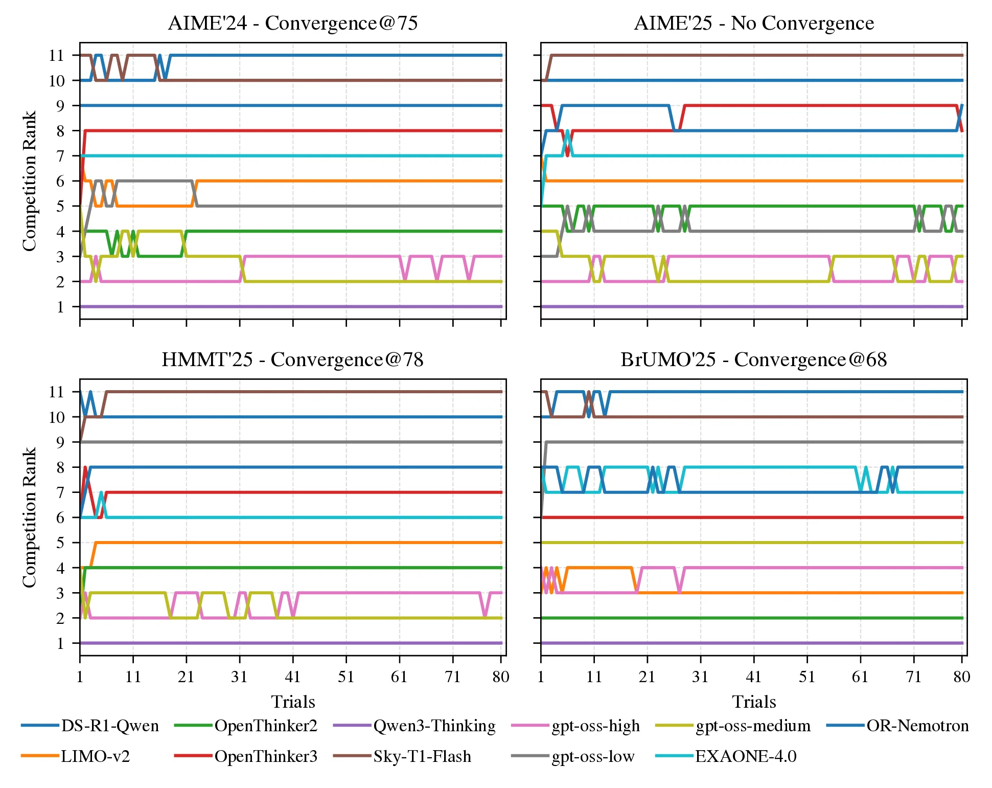
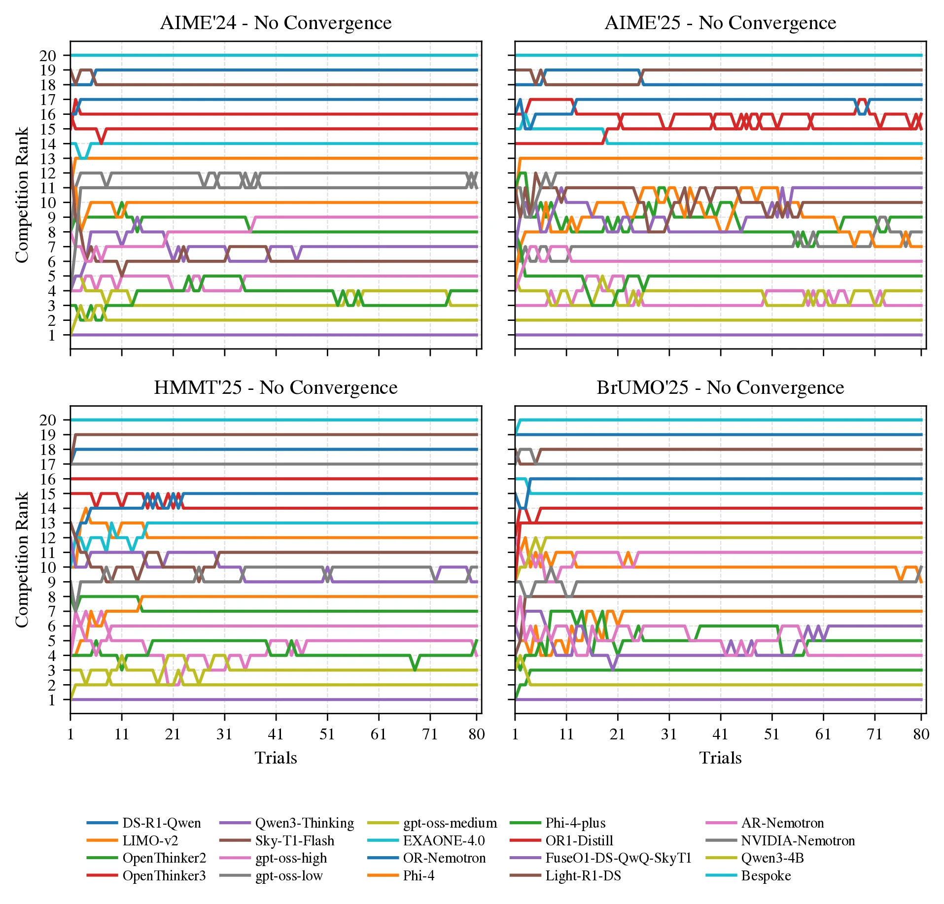
Worst-case scenarios
To further distinguish the Bayes@ framework from avg@, we analyze the worst-case bootstrap replicates, i.e., those that either require the maximum number of trials to stabilize the rankings or fail to converge. For 11 LLMs, Figure 8 shows these trajectories as competition rankings, with each line tracing a model’s rank as trials accumulate; convergence is defined as the point at which the ranking order remains unchanged for all subsequent trials. In AIME'24 the ranking converges at trial 75, in HMMT'25 at trial 78, and in BrUMO'25 at trial 68, whereas in AIME'25 no convergence is observed within 80 trials, underscoring persistent instability and the need for additional trials or Bayes@'s credible intervals. When a ranking does not converge within the trial budget (as for AIME'25 in Figure 1) only Bayes@ can be used to quantify uncertainty and estimate the minimum required for a reliable ranking (see Section 2.7.2).
This situation becomes even more severe as more models are included. As shown in Figure 9, when the number of models is increased to , none of the datasets exhibit convergence. To examine convergence as a function of more systematically, we consider a pool of 20 LLMs (Table 7) and construct 50 subsets of 5 models (?), 20 subsets of 10 models (?), and 20 subsets of 15 models (?). For each subset, we generate bootstrap replicates to estimate convergence@. Figure 6 reports the resulting convergence@ values across all subsets and replicates, showing that as the number of models increases, evaluation methods such as avg@ and the Pass@ family become unreliable for estimating model abilities and producing stable rankings.
Rubric-Aware Categorical Evaluation
While evaluation is often reduced to binary correctness, this simplification discards valuable signals that capture other aspects of model behavior. For instance, LLM outputs can be assessed not only on correctness but also on whether they are well-structured, coherent, or exhibit step-by-step reasoning in mathematical tasks. In practice, evaluators could record richer dimensions such as format compliance, calibration of confidence, degenerate outputs, out-of-distribution (OOD) behavior, and verifier scores. This limitation is especially important for reasoning models, where overthinking [44] inflates token usage without corresponding gains in reliability. Bayes@ provides a principled way to capture these richer outcomes. By treating per-item results as categorical rather than binary, the approach aligns more closely with actual goals while preserving statistical rigor and transparency.
Concretely, for each question and trial, a set of base signals is logged (e.g., correctness, presence of a boxed final answer, length, and perplexity features). These base signals are then augmented with probabilistic labels from a lightweight reward model (e.g., calibrated probabilities of correct, wrong, or off-task) [45]. From these signals, rubric variables are defined (Table 4) and different categorical schemata are instantiated (Table 5), mapping each attempt into one of categories. Under Bayes@, the resulting category counts induce a Dirichlet posterior, and a rubric is specified by the weight vector in algorithm 1. Different choices of schema and encode different evaluation preferences (e.g., stricter compliance, stronger penalties for confidently wrong answers, or efficiency-adjusted scoring). This procedure yields posterior means and credible intervals for each rubric.
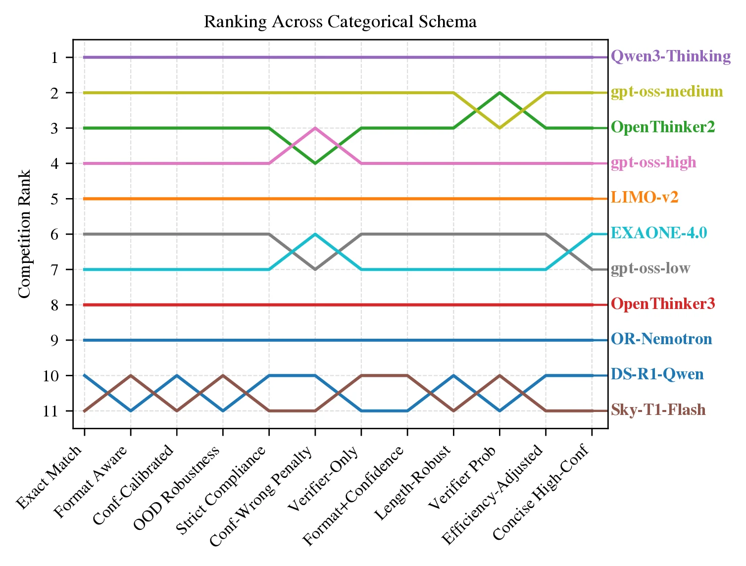
figure 10 summarizes aggregated results across tasks. The leader Qwen Qwen3-30B-A3B-Thinking-2507 ranks first under all selected schemata, but the gap to rank 2 depends on the rubric: it is largest under Conf-Wrong Penalty and smallest under Verifier-Only. Mid-pack reorderings are rubric-sensitive: under Verifier Prob, OpenThinker OpenThinker2-32B edges gpt-oss gpt-oss-20b_medium; under calibration-heavy schemata (e.g., Conf-Calibrated and Format+Confidence), gpt-oss gpt-oss-20b_high overtakes OpenThinker OpenThinker2-32B; and OOD Robustness narrows the gap between ranks 2 and 3. Several categories (Format Aware, Length-Robust, and Strict Compliance) agree closely, indicating that once correctness is accounted for, formatting and length rarely flip the top ranks. In contrast, calibration-focused categories emphasize and penalize confidently wrong behavior, and efficiency-oriented categories favor concision. The lower tier is stable across categories (EXAONE EXAONE-4.0-1.2B, OpenThinker OpenThinker3-1.5B, NVIDIA OpenReasoning-Nemotron-1.5B, Sky-T1-32B-Flash Sky-T1-32B-Flash, DeepSeek DeepSeek-R1-Distill-Qwen-1.5B), suggesting rubric choice primarily reshuffles the middle while preserving extremes. Overall, the categorical schemata surface complementary facets - format compliance, calibration, efficiency, OOD robustness, and verifier alignment - making rubric-dependent differences explicit and enabling compute-efficient, uncertainty-aware comparisons aligned with evaluation goals. For a comprehensive discussion of the categorical Bayesian evaluation framework, including base signals, schema definitions, and their impact on model rankings, see Appendix 13.
Related Work
Functional-correctness evaluation with Pass@ became standard in code generation with HumanEval (OpenAI Codex): generate samples, a task is solved if any sample passes unit tests, and estimate the overall rate with an unbiased estimator that requires producing samples per task [24]. Although Pass@ was initially introduced in the context of coding, it later became the de facto choice to evaluate LLMs not only on math reasoning tasks [46, 47, 48, 49, 50, 51, 52, 53, 27, 54] but also on safety evaluations spanning agent red-teaming, jailbreaks, and backdoor analyses [55, 56, 57, 58, 59, 60]. For a broader review of these metrics and their variants, see Appendix 15. Beyond standard Pass@, pass^ quantifies reliability across i.i.d. trials for agents, while the generalized G-pass@k continuum (and its area-under- summary mG-Pass) jointly assess potential and stability in reasoning outputs [61, 27].
Efforts like HELM advance holistic, transparent evaluation across scenarios and metrics [5], while practice guidelines distill reproducibility pitfalls and prescribe multi-run, uncertainty-aware reporting with fixed prompts, decoding, and dataset [62]. The LM Evaluation Harness offers standardized, reproducible frameworks to implement these recommendations [62]. It supports uncertainty reporting through binomial-style uncertainty estimates for binary mean metrics and bootstrap estimates for others.
The last category of related work focuses on measuring uncertainty in LLM evaluation. These works converge on interval-aware, small-sample-valid reporting rather than CLT/Wald error bars. Bowyer et al. show that CLT-based intervals miscalibrate on small benchmarks and advocate small--appropriate frequentist or Bayesian intervals for reliable comparisons [42]. A Bayesian alternative models capability as a latent success probability and reports posterior uncertainty that remains informative with limited trials, yielding more stable rankings [34]. In judge-based settings, Judging LLMs on a Simplex places model and judge behavior on the probability simplex, enabling uncertainty-aware comparisons and highlighting how distributional structure matters for evaluation [63]. Beyond bespoke LLM metrics, prediction-powered inference supplies general procedures for valid confidence intervals that leverage model predictions to reduce labeled-sample requirements [64]. Finally, in adjacent retrieval evaluation with LLM-generated assessments, Oosterhuis et al. construct reliable confidence intervals and demonstrate that calibrated uncertainty, rather than point estimates, should guide decisions, reinforcing this shift for LLM evaluation more broadly [65].
Conclusion: Strengths, Limitations & Future Directions
The overall benefits of the Bayesian framework are summarized in Table 3: it provides fast convergence, analytical uncertainty estimates, and the incorporation of prior knowledge and categorical results. However, it is worth noting that our approach quantifies statistical uncertainty from finite samples; it does not fix dataset bias, distribution shift, or rubric misspecification. Results therefore depend on the chosen benchmark, prompts, and inference settings (hardware). Although we have validated our approach with biased-coin LLM mimic simulations, together with experiments using actual LLMs (up to trials across four tasks and 20 models), more extensive evaluations may be constrained by computing and academic budgets.
The focus of the current work was the simplest version of the Bayesian approach, using a uniform prior, which provides a conservative and reproducible starting point. But the theory allows for more complex, informative priors, and this opens up a rich vein of future directions that should be systematically explored: for example priors from past runs, domain- or task-conditioned priors, and expert-elicited priors. These have the potential of accelerating convergence even further, but must be chosen and reported carefully. Clear guidance and tools for prior elicitation will hopefully ensure that gains in sample efficiency do not come at the cost of hidden bias.
Ethics Statement
This research relies only on publicly available, non-personal benchmarks; no human subjects, user data, or PII are involved. Potential misuse includes cherry-picking priors, rubrics, or samples to exaggerate performance. To prevent this, use of Bayes@ with user-defined priors requires clear documentation and reporting of posterior credible intervals.
Reproducibility Statement
To ensure reproducibility, detailed implementation instructions are provided in Appendix 16.
Acknowledgments
This research was supported in part by NSF awards 2117439, 2112606, and 2320952.
Appendix
Derivation of Bayesian Estimator and Uncertainty
As described in the main text, the Bayesian framework is built on two quantities. The first is , the average of over the joint posterior for all the questions:
where the integration region is the probability simplex defined as the set of all possible -dimensional vectors such that . The second is the variance associated with our Bayesian estimator,
Our derivation of closed-form expressions for and builds on the generalized () and original () Laplace rule of succession theory from [41], recovering those results in the special case of a single question (). We start with Bayes' rule for each row of :
The likelihood is a -category multinomial distribution over trials, with the probability distribution function:
where , is the vector with elements , and is the Kronecker delta.
The prior is chosen as the conjugate prior of the multinomial, a Dirichlet distribution , with concentration parameter vector . [35] A uniform prior (no prior knowledge) sets for all . Prior information from an earlier matrix (with as the category for the th trial of the th question) can be incorporated as:
The Dirichlet prior is:
where .
The normalization constant is:
and since the Dirichlet is the conjugate prior, the posterior is , with . The posterior distribution is:
where .
The moment generating function is:
where , and .
Each integral is the moment-generating function for a Dirichlet distribution, expressed via the confluent Lauricella hypergeometric function :
where
and is the Pochhammer symbol.
The moments are:
Expanding to :
Substituting into equation 11 and computing derivatives yields:
The algorithm summarizing this calculation is shown in Algorithm 1 in the main text.
Proof of Equivalence of Bayesian and Average Rankings for Uniform Prior
For Bayesian estimators using a uniform prior (where , , ), the expression for the mean from equation 15 simplifies as:
where the constant is given by
and . Here, relates to a naive weighted average accuracy over the number of answers in each category,
via
Note that in the binary case where , , , the value of is just regular average accuracy avg@. For categorical cases, it is just a weighted generalization of avg@.
Since is constant across models and the prefactor is positive, we see that if , the corresponding values of and from the two methods must always give the same ranking, . Additionally, in the limit of a large number of trials, , we see that and , as expected.
This equivalence extends to uncertainty quantification. The relationship between the standard deviation of the average () and the Bayesian standard deviation ( from equation 15) is
The Bayesian expression for is valid for all and , providing a reliable method to compute uncertainty in avg@ without relying on the Central Limit Theorem.
Runtime
To see the asymptotic runtime and memory scaling let:
From Algorithm 1, the work is:
So the overall time complexity is:
i.e., linear in the number of entries in the result matrices and linear in the number of categories.
The memory footprint is likewise linear:
Note that the evaluation consists of tallying counts and then plugging them into closed-form expressions for and ; no iterative optimization or Monte Carlo sampling is required.
Categorical Evaluation
Rubric-aware Bayes@N Evaluation of Reasoning Models
As discussed in Section 2.3, Section 3.4, for each question , every attempt yields base signals such as has_box, is_correct, token_ratio, prompt_bpt, completion_bpt, and verifier probabilities compass_context_A, compass_context_B, and compass_context_C for correct, wrong, and invalid/off-task. Using thresholds and Boolean criteria, each attempt is mapped into one of categories under a chosen schema (e.g., Format Aware, Conf-Wrong Penalty, Efficiency-Adjusted; Table 5). We instantiate categorical schemata and update posterior means via Dirichlet-multinomial inference, yielding metrics that preserve correctness while explicitly reflecting formatting, calibration, and efficiency.
Base signals
All signals are directly obtainable from common LLM inference stacks such as Hugging Face transformers [66] and vLLM [16], via per-step scores/log-probs and termination metadata, and require no model-specific instrumentation; the verifier probabilities compass_context_A, compass_context_B, and compass_context_C are defined in Section 13.1.2.
- has_box: 1 if a final boxed answer is present; else 0.
- is_correct: 1 if the answer is correct; else 0.
- token_ratio: completion tokens normalized by 32,768.
- repeated_pattern: 0 if
finish_reasonisstop; else 1 (degenerate output). - prompt_bpt: negative average prompt log-prob in bits/token (lower is better).
- completion_bpt: negative average completion log-prob in bits/token (lower is better).
- compass_context_A: verifier contextual probability of correct.
- compass_context_B: verifier contextual probability of wrong.
- compass_context_C: verifier contextual probability of irrelevant/off-task.
Reward models in evaluation.
While reward models are most familiar from fine-tuning (e.g., RLHF), we use one as a lightweight verifier to supply per-attempt label probabilities for
in evaluation. Concretely, we employ OpenCompass CompassVerifier-3B to produce probabilities and then apply contextual calibration to obtain a more robust, prompt-stable label distribution: we evaluate next-token scores for the candidate labels at a fixed answer slot, subtract a content-free baseline logit from the task logit for each label , and apply temperature scaling to yield calibrated probabilities
This helps us mitigate saturation and the entanglement of formatting and confidence seen with last-token probabilities, and improves probability calibration for downstream rubric scoring.
Selected categorical schema.
We define 12 schemata (Table 5) using the rubric variables (Table 4) derived from the base signals; here are two illustrative definitions (the others follow analogously):
- Format Aware: \[ cat = cases 0 & invalid \\ 1 & wrong unboxed \\ 2 & wrong boxed \\ 3 & correct unboxed \\ 4 & correct boxed cases \]
- Conf-Wrong Penalty: \[ cat = cases 0 & invalid \\ 1 & wrong_high_conf \\ 2 & wrong low_conf \\ 3 & correct cases \]
Rubric weights are chosen to reflect evaluation preferences. For example, Format Aware might use to mildly reward formatting when correct and slightly penalize confidently wrong (via schema choice); Efficiency-Adjusted can downweight verbose outputs among both correct and wrong categories.
- Exact Match Correctness only; ignores formatting, confidence, and length.
- Format Aware Rewards boxed, well-formatted answers; distinguishes boxed/unboxed even when wrong.
- Conf-Calibrated Penalizes confidently wrong; grades correct answers by confidence (low/mid/high).
- OOD Robustness Separates in-distribution vs. OOD prompts; checks correctness under both.
- Strict Compliance Requires boxed final answers; unboxed-correct is treated as non-compliant.
- Conf-Wrong Penalty Heavier penalty for wrong answers at high confidence; lighter when uncertain.
- Verifier-Only Uses verifier signals alone to rank; model-agnostic prob of the verifier.
- Format+Confidence Balanced composite over (boxed/unboxed) (low/high confidence) for both wrong and correct; emphasizes boxed, high-confidence correctness and penalizes confidently wrong.
- Length-Robust Isolates correctness irrespective of verbosity; does not penalize length.
- Verifier Prob Probes agreement with the verifier: flags wrong with high verifier A as inconsistent and distinguishes under/over-confidence on correct.
- Efficiency-Adjusted Rewards short, correct completions; penalizes verbose outputs (especially when wrong).
- Concision-High-Conf Prefers concise, high-confidence correct answers; downweights verbose correctness.
| lll@ Rubric variables | Formula | Description |
|---|---|---|
| invalid | Category 0 reserved for invalid. | |
| correct | Boolean mask of correctness. | |
| wrong | Complement of correct. | |
| high_conf | Confidence proxy | |
| low_conf | Complement of high_conf. | |
| wrong_high_conf | wrong | Penalize confidently wrong. |
| ood | Out-of-distribution prompt. | |
| ind | In-distribution prompt. | |
| economical | Short completions. | |
| moderate | Medium-length completions. | |
| verbose | Long completions. | |
| boxed | Answer is boxed. | |
| unboxed | Answer is not boxed. | |
| A_high | Verifier confidence high. | |
| 40th percentile of | ||
| 60th percentile of among wrong items | ||
| 90th percentile of | ||
| 33rd and 66th percentiles of | ||
| 33rd and 66th percentiles of correct items |
| Categorical Schema | Rubric |
|---|---|
| Exact Match | 0 invalid; 1 wrong; 2 correct |
| Format Aware | 0 invalid; 1 wrong unboxed; 2 wrong boxed; 3 correct unboxed; 4 correct boxed |
| Conf-Calibrated | 0 invalid; 1 wrong low_conf; 2 wrong_high_conf; 3 correct low_conf; 4 correct mid; 5 correct high_conf |
| OOD Robustness | 0 invalid; 1 ood wrong; 2 ind wrong; 3 ood correct; 4 ind correct |
| Strict Compliance | 0 invalid; 1 wrong (correct unboxed); 2 correct boxed |
| Conf-Wrong Penalty | 0 invalid; 1 wrong_high_conf; 2 wrong low_conf; 3 correct |
| Verifier-Only | 0 invalid; 1 high C; 2 high B; 3 A_high |
| Format+Confidence | 0 invalid; 1 wrong unboxed; 2 wrong boxed low_conf; 3 wrong boxed high_conf; 4 correct unboxed low_conf; 5 correct unboxed high_conf; 6 correct boxed low_conf; 7 correct boxed high_conf |
| Length-Robust | 0 invalid; 1 wrong; 2 correct |
| Verifier Prob | 0 invalid; 1 wrong A_high; 2 wrong A_high; 3 correct A_high; 4 correct A_high |
| Efficiency-Adjusted | 0 invalid; 1 wrong economical; 2 wrong moderate; 3 wrong verbose; 4 correct economical; 5 correct moderate; 6 correct verbose |
| Concision-High-Conf | 0 invalid; 1 wrong; 2 correct verbose; 3 correct moderate; 4 correct economical; 5 correct economical high_conf |
Domain-agnostic rubric-aware Bayes@N
The Bayesian construction is intentionally domain-agnostic: it applies whenever model outputs can be mapped into a finite set of categories equipped with a rubric. The evaluator specifies
- a mapping from raw outputs (and any side information) to categorical labels , and
- a weight vector that encodes how those categories are valued.
Given these choices, Bayes@N returns the posterior mean as a rubric-aware point estimate, and as an uncertainty estimate, for any such categorical evaluation.
This viewpoint naturally covers subjective tasks. For instance:
- In summarization, each response could be rated or by multi-criteria scores such as faithfulness, coverage, style, and harmful content. Each discrete level becomes a category index , and reflects the importance of that level or criterion.
- In dialogue safety, categories might distinguish , or finer-grained notions such as policy violations vs. merely over-cautious refusals.
Once the labels are available (from humans or an LLM-as-a-judge), Bayes@N provides Bayesian estimates and credible intervals for any chosen rubric-based score, reusing the same closed-form posterior as in the binary case.
Two aspects are particularly promising for future work in such subjective domains:
- Preference-based evaluation with rubrics. When model comparisons are driven by preferences (either from human experts or LLM judges), each comparison can be converted into categorical labels over rubric dimensions (e.g., faithfulness, verbosity, harmfulness). A downstream weight vector can then fold these dimensions into a single scalar score that reflects application-specific trade-offs.
- Transferring prior evidence across related tasks. The optional prior matrix in Algorithm 1 lets us encode earlier outcome frequencies as a Dirichlet prior. For example, if a summarization system has been evaluated on a news dataset, the empirical category counts on that dataset can serve as prior counts when evaluating a closely related dataset. This allows stable rubric distributions to be reused across adjacent tasks or benchmark revisions, while still updating with new data.
An important limitation in subjective settings is that Bayes@N does not resolve disagreement or bias in the rubric or labeling process itself. The framework assumes a labeling scheme (from humans or an LLM-based judge) and a weight vector are given; it then provides a statistically principled way to aggregate those labels and quantify uncertainty. Designing good rubrics and calibrating judges remain separate modeling decisions.
Scorio
Alongside this paper, we release Scorio, an open-source Python package that implements the evaluation framework presented in this work. Scorio provides a simple, unified API for computing Bayes@, avg@, Pass@, and their credible intervals, enabling researchers to adopt principled Bayesian evaluation with minimal effort. The package is available on PyPI and its documentation is hosted at https://scorio.readthedocs.io.
Installation.
Scorio can be installed via:
pip install scorioBasic usage.
All evaluation functions operate on a results matrix , where is the number of problems, is the number of trials per problem, and is the number of outcome categories. An optional weight vector of length maps each category to a score. Listing 2 shows binary evaluation using both the Bayesian estimator and Pass@.
Scorio.import numpy as np
from scorio import eval
# Binary outcomes: M=2 problems, N=5 trials each
R = np.array([[0, 1, 1, 0, 1],
[1, 1, 0, 1, 1]])
# Bayesian evaluation (binary: w defaults to (0, 1))
mu, sigma = eval.bayes(R)
print(f"Bayes@5: mu={mu:.4f}, sigma={sigma:.4f}")
# Average accuracy
a, sigma_a = eval.avg(R)
print(f"avg@5: mu={a:.4f}, sigma={sigma_a:.4f}")
# Pass@k
print(f"Pass@1 = {eval.pass_at_k(R, k=1):.4f}")
print(f"Pass@2 = {eval.pass_at_k(R, k=2):.4f}")Credible intervals.
Each estimator has a companion _ci function that returns the posterior mean, standard deviation, and a credible interval, as shown in Listing 3.
# 95
mu, sigma, lo, hi = eval.bayes_ci(R, confidence=0.95)
print(f"Bayes@5: {mu:.4f} [{lo:.4f}, {hi:.4f}]")

# 95
mu, sigma, lo, hi = eval.pass_at_k_ci(R, k=1)
print(f"Pass@1:  {mu:.4f} [{lo:.4f}, {hi:.4f}]")
Categorical (rubric-based) evaluation.
For graded outcomes with categories, a weight vector specifies the score associated with each category. Listing 4 illustrates evaluation under a three-level rubric () with partial credit.
# Graded outcomes: 0=incorrect, 1=partial, 2=correct
R = np.array([[0, 2, 1, 0, 2],
              [2, 1, 1, 2, 1]])

# Weight vector: incorrect=0, partial=0.5, correct=1
w = np.array([0.0, 0.5, 1.0])

mu, sigma = eval.bayes(R, w)
print(f"Bayes@5 (graded): mu={mu:.4f}, sigma={sigma:.4f}")

mu, sigma, lo, hi = eval.bayes_ci(R, w, confidence=0.95)
print(f"95
Incorporating prior evidence.
When prior evaluation data are available (e.g., from a previous benchmark or a pilot study), they can be passed as a prior matrix to inform the posterior, as described in Section 2.7.1. Listing 5 shows a minimal example in which a short pilot run is reused as prior evidence for a new evaluation.
# Prior outcomes from a pilot study (M=2, D=3 trials)
R0 = np.array([[1, 0, 1],
               [0, 1, 0]])

mu, sigma = eval.bayes(R, w=None, R0=R0)
print(f"Bayes@5 (with prior): mu={mu:.4f}, sigma={sigma:.4f}")
Table 6 summarizes the main Scorio API.
Scorio evaluation API. All functions accept a results matrix . Functions with the _ci suffix additionally return a credible interval.| lll@ Function | Returns | Description |
|---|---|---|
bayes(R, w, R0) | Bayesian posterior mean and uncertainty | |
bayes_ci(R, w, R0) | + credible interval | |
avg(R, w) | Weighted average and uncertainty | |
avg_ci(R, w) | + credible interval | |
pass_at_k(R, k) | Pass@ estimate | |
pass_at_k_ci(R, k) | + credible interval | |
pass_hat_k(R, k) | Pass\^ | |
g_pass_at_k_tau(R, k, tau) | G-Pass@ | |
mg_pass_at_k(R, k) | mG-Pass@ |
Extended Related Work
The evaluation of LLMs in generative reasoning tasks, under test-time scaling (e.g., via repeated sampling[67]), has evolved to address the stochastic nature of inference and the need for robust measures of functional correctness. Early approaches relied on syntactic similarity metrics like BLEU [68] and CodeBLEU [69], which compare generated answers against reference solutions. However, these metrics often fail to capture semantic correctness in reasoning tasks, motivating metrics based on execution-validation or test-based validation [70, 69]. This limitation has shifted focus toward functional evaluation, where the generated solution is assessed via a ground truth to verify correctness[70, 71]. In this section, we review key functional metrics, focusing on those that leverage multiple samples to scale performance at inference time. These metrics form the basis to assess LLM capabilities but often overlook probabilistic uncertainty or consistency across samples, motivating our novel Bayesian framework.
The Pass@ metric, originally introduced by [70, 24] for evaluating LLMs trained on code. It measures the probability that at least one of independently generated samples for a given problem passes all associated unit tests (i.e., by matching ground-truth answers or satisfying logical constraints), offering a practical estimate of a model's potential performance in solving a variety of complex tasks and problems. The unbiased estimator of Pass@ is computed as:
where is the total number of generated samples and is the total number of correct solutions within the trials. This estimator has smaller uncertainty in the limit of , ensuring reliable approximations. However, due to computational costs, is often comparable to in practice, which can increase variance and weaken evaluation stability. The Pass@ metric has been adapted beyond code to evaluate LLMs in various tasks requiring verifiable correctness, such as math, logic, and general reasoning [71, 72, 73, 74].
Pass^, introduced in [61], extends the Pass@ metric to capture both the potential performance and the consistency of LLMs in reasoning tasks, where evaluating the reliability and stability of generated solutions is crucial. Pass^ is defined as the probability that all trials are correct:
where and retain the same meanings as in Pass@. This metric assumes that all the trials are independent and uniformly distributed, approximating the binomial distribution with a hypergeometric distribution to account for sampling without replacement. By requiring all samples to be correct, Pass^ provides a stringent measure of model consistency and stability.
To introduce flexibility, [27] proposed G-Pass@, which incorporates a tolerance threshold :
where is the smallest integer greater than or equal to . This formulation allows up to incorrect solutions, balancing the assessment of potential with consistency. As a special case, Pass@ corresponds to G-Pass@ in the limit .
Furthermore, [27] introduced mG-Pass@, an interpolated metric that integrates G-Pass@ over :
providing a more comprehensive measure that jointly reflects performance potential and reasoning stability.
These extended metrics have been applied to mathematical reasoning benchmarks such as LiveMathBench, MATH, and AIME, where they reveal substantial performance degradation of LLMs under stricter stability requirements.
Experiment Setup and Reproducibility
Metrics
Kendall's Tau:
Kendall's tau () [75] is a nonparametric rank correlation coefficient that quantifies the ordinal relationship between two ranked sets by evaluating the consistency in their orderings. For two rankings of items, it examines all unique pairs where :
- A pair is concordant if the relative ordering of items and is the same in both rankings (both place before or vice versa).
- A pair is discordant if the relative ordering is different.
- Pairs with ties in either ranking are neither concordant nor discordant.
Define as the number of concordant pairs, as the number of discordant pairs, and as the total number of unique pairs. Let represent the number of tied pairs in the first ranking, and similarly for the second ranking. The two common variants are the following:
Tau-a assumes no ties and may underestimate correlation when ties occur. Tau-b, which corrects for ties, is better suited for datasets with equivalent rankings.
In our implementation, we use scipy.stats.kendalltau with its default variant='b', which computes efficiently and handles ties appropriately. The coefficient ranges from (perfect disagreement) to (perfect agreement), with indicating no association. This metric provides a robust, distribution-free measure for comparing model performance rankings, particularly when ties reflect meaningful equivalences.
Convergence@.
For a given bootstrap replicate, we measure convergence in terms of an exact ranking match. At each step , we compute the ranking induced by the first trials and compare it to a gold-standard ranking (obtained from all trials). We then define
and refer to as the convergence@ value for that replicate. If no such exists, we declare that replicate to exhibit no convergence.
Models and Datasets
Datasets.
We evaluate on four math-reasoning test sets: AIME'24 [25], AIME'25 [26], BrUMO'25 [37], and HMMT'25 [36]. AIME is administered by the Mathematical Association of America and consists of two sets of 15 integer-answer problems; we use the 2024 and 2025 problem sets. For HMMT'25, we use the officially posted February 2025 contest set (algebra, geometry, number theory, and combinatorics). For BrUMO'25, we use the published 2025 problem sets from the tournament archive.
Models.
Unless noted otherwise, we run each generator with the provider-recommended chat template (DeepSeek/Qwen style when unspecified) and identical decoding settings (below) to minimize template-induced variance. The base model cohort includes 11 models (8 distinct models + 3 modes (low, medium, and high) of gpt-oss) as follows: Sky-T1-32B-Flash Sky-T1-32B-Flash [76] (reasoning-optimized “flash” variant tied to overthinking-reduction work), Qwen Qwen3-30B-A3B-Thinking-2507 [77] (Qwen3 series, reasoning variant), DeepSeek DeepSeek-R1-Distill-Qwen-1.5B [46] (distilled reasoning model), gpt-oss gpt-oss-20b [78] (OpenAI open-weight reasoning model; we use the default quantization, MXFP4, and, for prompting, rely on OpenAI Harmony, which defines three levels of reasoning effort), LIMO LIMO-v2 [79] (data-efficient reasoning fine-tuned on curated traces), EXAONE EXAONE-4.0-1.2B [80] (hybrid non-reasoning/reasoning modes), NVIDIA OpenReasoning-Nemotron-1.5B [81, 82, 83, 84] (open-weight small reasoning model), OpenThinker OpenThinker2-32B [85] and OpenThinker OpenThinker3-1.5B [85] (trained on OpenThoughts2/3 data recipes).
To investigate the effect of the number of models required to reach a stable ranking with and without credible intervals, in addition to the 11 above-mentioned models, we extend the evaluation to 20 models in total (17 + 3): Microsoft Phi-4-reasoning and Microsoft Phi-4-reasoning-plus [86] (14B small language models with supervised “teachable” reasoning traces and an RL-enhanced variant), OpenR1 OpenR1-Distill-7B [87] (an open 7B distillation of DeepSeek-R1 using fully public data), FuseO1 FuseO1-DeepSeekR1-QwQ-SkyT1-Flash-32B-Preview [88] (System-II “long-short” reasoning fusion of DeepSeek-R1, QwQ, and Sky-T1-32B-Flash), Light-R1 Light-R1-14B-DS [89] (a Qwen2.5-based long-chain-of-thought model further improved with GRPO-style reinforcement learning), NVIDIA AceReason-Nemotron-1.1-7B [90] (7B NVIDIA Nemotron math/code model trained on OpenMathReasoning/OpenCodeReasoning data), NVIDIA NVIDIA-Nemotron-Nano-9B-v2 [91] (a hybrid Mamba-Transformer “Nano 2” model with controllable reasoning mode), Qwen Qwen3-4B-Thinking-2507 [77] (4B “thinking” variant of Qwen3 with scaled reasoning depth), and Bespoke-Stratos Bespoke-Stratos-7B [92] (Qwen2.5-7B student obtained via DeepSeek-R1-based reasoning distillation on Bespoke-Stratos-17k).
For verification, we additionally use CompassVerifier CompassVerifier-3B [45], a lightweight answer verifier suitable for outcome reward and equivalence checking.
| ID | Model | Short name |
|---|---|---|
| 1 | DeepSeek DeepSeek-R1-Distill-Qwen-1.5B | DS-R1-Qwen |
| 2 | LIMO LIMO-v2 | LIMO-v2 |
| 3 | OpenThinker OpenThinker2-32B | OpenThinker2 |
| 4 | OpenThinker OpenThinker3-1.5B | OpenThinker3 |
| 5 | Qwen Qwen3-30B-A3B-Thinking-2507 | Qwen3-Thinking |
| 6 | Sky-T1-32B-Flash Sky-T1-32B-Flash | Sky-T1-Flash |
| 7 | gpt-oss gpt-oss-20b_high | gpt-oss-high |
| 8 | gpt-oss gpt-oss-20b_low | gpt-oss-low |
| 9 | gpt-oss gpt-oss-20b_medium | gpt-oss-medium |
| 10 | EXAONE EXAONE-4.0-1.2B | EXAONE-4.0 |
| 11 | NVIDIA OpenReasoning-Nemotron-1.5B | OR-Nemotron |
| 12 | Microsoft Phi-4-reasoning | Phi-4 |
| 13 | Microsoft Phi-4-reasoning-plus | Phi-4-plus |
| 14 | OpenR1 OpenR1-Distill-7B | OR1-Distill |
| 15 | FuseO1 FuseO1-DeepSeekR1-QwQ-SkyT1-Flash-32B-Preview | FuseO1-DS-QwQ-SkyT1 |
| 16 | Light-R1 Light-R1-14B-DS | Light-R1-DS |
| 17 | NVIDIA AceReason-Nemotron-1.1-7B | AR-Nemotron |
| 18 | NVIDIA NVIDIA-Nemotron-Nano-9B-v2 | NVIDIA-Nemotron |
| 19 | Qwen Qwen3-4B-Thinking-2507 | Qwen3-4B |
| 20 | Bespoke-Stratos Bespoke-Stratos-7B | Bespoke |
Prompting.
For most models, we follow the provider-recommended DeepSeek/Qwen-style prompt: "Please reason step by step, and put your final answer within boxed\\." For gpt-oss gpt-oss-20b, we instead use the OpenAI Harmony prompt template, which provides three levels of reasoning effort. For NVIDIA OpenReasoning-Nemotron-1.5B, we adopt the task-specific prompt: "Solve the following math problem. Make sure to put the answer (and only the answer) inside boxed\\."
Reproducibility
Sampling setup. All trials use top- sampling with temperature, , batch size, and seeds -. We perform trials per dataset model.
Verifier. We use CompassVerifier CompassVerifier-3B as a reward model. During evaluation, we leverage the model's scores on prompts generated by other models to create categorical schemas. We rely on the Transformers [66] and Accelerate [93] libraries. To maximize throughput, we enable FlashAttention kernels [23] and adopt the DFloat11 format [94].
Serving stack. Token generation is served with vLLM (PagedAttention) [16], and models are loaded in bf16 unless the release requires MXFP4 (e.g., gpt-oss). We record log-probabilities for both the input prompt and generated tokens, and cap max_tokens at .
Hardware. All runs execute on clusters with NVIDIA H200 (141GB).
Computational Cost and Token Statistics
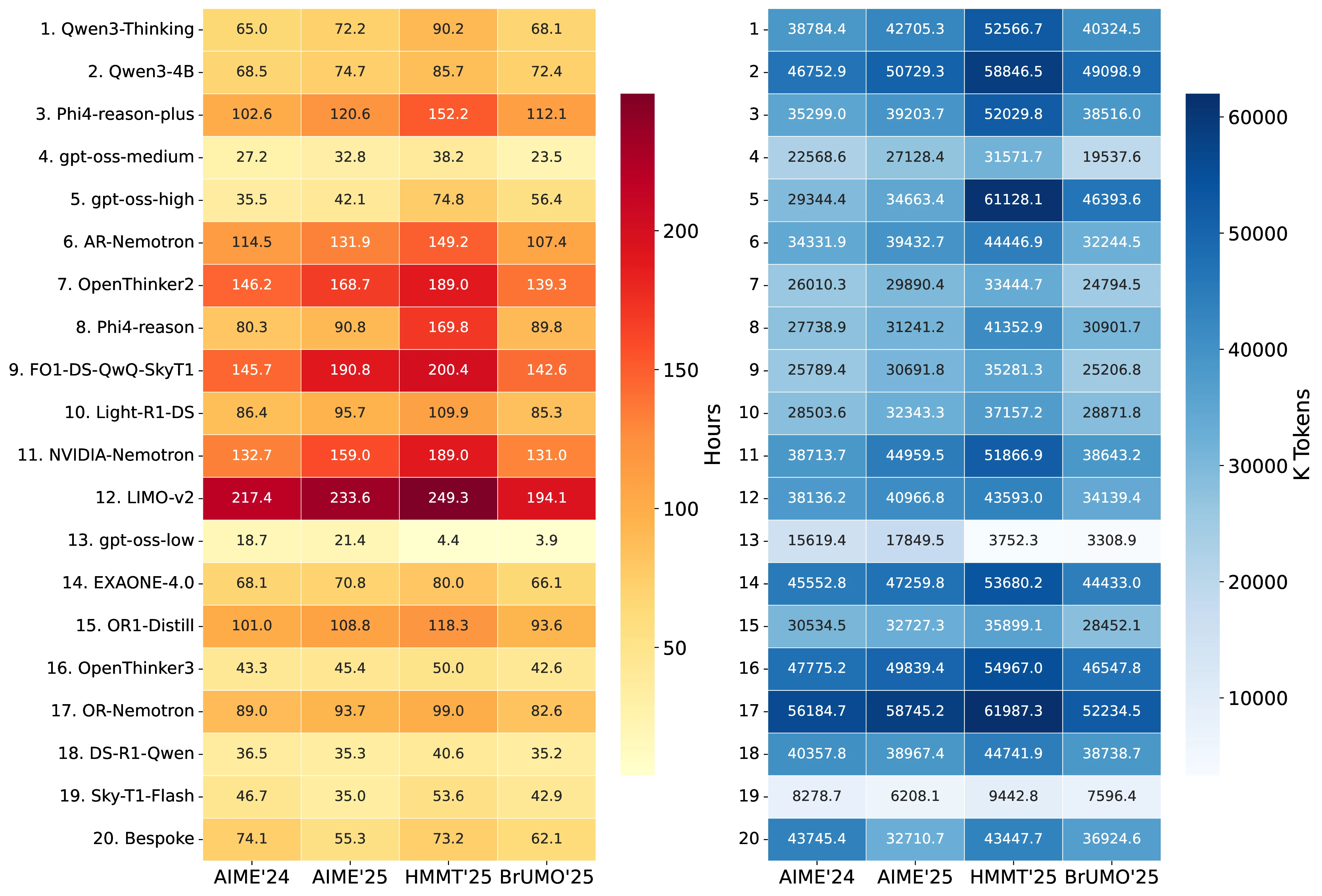
Across all tasks, we evaluated 20 models with 80 trials per model and 30 questions per benchmark, yielding a total of 192,000 independent inference runs. This required 7,445 GPU-hours (310 GPU-days) and generated 2.96B tokens (2,963,318,176) in total (see Figure 7 for details).
Task-level computational cost.
| Task | Inference Time (hours) | Completion Tokens (M) |
|---|---|---|
| AIME'24 | 1,699.4 | 680.0 |
| AIME'25 | 1,878.4 | 728.3 |
| HMMT'25 | 2,216.5 | 851.2 |
| BrUMO'25 | 1,650.9 | 666.9 |
| TOTAL | 7,445.2 | 2,926.4 |
HMMT'25 is the most expensive benchmark in terms of GPU time (2,217 GPU-hours), while BrUMO'25 is the least expensive (1,651 GPU-hours). Figure 7 provides a complementary visualization of these patterns, showing inference time and completion-token usage across models and tasks.
Token breakdown.
Aggregating across all tasks and models, the total number of tokens (prompt + completion) is 2.96B. The breakdown is:
- Prompt tokens: 37M (1.2%)
- Completion tokens: 2.93B (98.8%)
- Average per query: 15,434 tokens
GPU-hours by model efficiency.
The 20 model configurations varied substantially in computational efficiency:
- Most efficient:
gpt-oss-20b-low(48.4 GPU-hours for 9,600 queries) - Least efficient:
LIMO-v2(894.3 GPU-hours for 9,600 queries) - Average per query over all models: 139.6 seconds (2.3 minutes)
Convergence
While Figure 1 shows the PMF of convergence@, Figure 11 shows the corresponding cumulative distribution functions (CDFs). For Pass@ and Pass@, there is no convergence, as the figure shows no CDFs associated with them. The CDFs are computed using the same bootstrap replicates as in Figure 1. The distribution of convergence@ is computed using the result matrices from the first 11 models (Table 7). Among the replications, Figure 8 shows the worst-case scenarios in which convergence@ attains its maximum value. As discussed in Section 3.3.1, convergence@ depends on the number of models : as increases, convergence@ grows. When we extend the pool of LLMs from 11 to 20 models, convergence@ reaches no convergence for all datasets (see Figure 9).
To complement the worst-case trajectories discussed in Section 3.3.1 and shown in Figure 8, Figure 9, we provide additional details on the construction of the model subsets and the resulting convergence behavior. Table 7 lists the pool of 20 LLMs used in this analysis, together with the shortened identifiers that appear throughout the figures and tables. From this pool we construct 50 subsets of 5 models, 20 subsets of 10 models, and 20 subsets of 15 models, as summarized in ?, ?, ?. Each row in these tables corresponds to one subset, indicating which models are included and reporting, under each task, the convergence@ metric computed without a credible interval; each entry is the mean over bootstrap replicates. Thus, the tables make explicit how convergence@ depends not only on the task but also on the particular mixture of models being compared. Aggregating across all subsets and replicates, Figure 6 then visualizes the distribution of convergence@ as a function of the number of models , confirming the trend anticipated in the main text: as grows from 5 to 15 and ultimately to the full set of 20 LLMs, the required number of trials increases and non-convergence becomes common, indicating that rank-based evaluation methods such as avg@ and the Pass@ family become increasingly unreliable without an accompanying Bayesian uncertainty quantification such as Bayes@.
tables/comb5 tables/comb10 tables/comb15
References
- Attention Is All You Need. Advances in Neural Information Processing Systems. 2017. https://arxiv.org/abs/1706.03762
- Language Models are Few-Shot Learners. Advances in Neural Information Processing Systems. 2020. https://proceedings.neurips.cc/paper/2020/file/1457c0d6bfcb4967418bfb8ac142f64a-Paper.pdf
- Stack Overflow Developer Survey 2025: AI and Developer Tools. misc. 2025. https://survey.stackoverflow.co/2025/ai
- Artificial Intelligence Index Report 2025. arXiv preprint arXiv:2504.07139. 2025. https://arxiv.org/abs/2504.07139
- Holistic Evaluation of Language Models. arXiv preprint arXiv:2211.09110. 2022. https://arxiv.org/abs/2211.09110
- Measuring Massive Multitask Language Understanding. International Conference on Learning Representations (ICLR). 2021. https://arxiv.org/abs/2009.03300
- Beyond the Imitation Game: Quantifying and Extrapolating the Capabilities of Language Models (BIG-bench). arXiv preprint arXiv:2206.04615. 2022. https://arxiv.org/abs/2206.04615
- Scaling Laws for Neural Language Models. arXiv preprint arXiv:2001.08361. 2020. https://arxiv.org/abs/2001.08361
- Training Compute-Optimal Large Language Models. arXiv preprint arXiv:2203.15556. 2022. https://arxiv.org/abs/2203.15556
- Chain-of-Thought Prompting Elicits Reasoning in Large Language Models. Advances in Neural Information Processing Systems. 2022. https://openreview.net/forum?id=%5FVjQlMeSB%5FJ
- Training language models to follow instructions with human feedback. Advances in Neural Information Processing Systems. 2022. https://proceedings.neurips.cc/paper%5Ffiles/paper/2022/file/b1efde53be364a73914f58805a001731-Paper-Conference.pdf
- LLM.int8(): 8-bit Matrix Multiplication for Transformers at Scale. misc. 2022. https://arxiv.org/abs/2208.07339
- GPTQ: Accurate Post-Training Quantization for Generative Pre-trained Transformers. misc. 2022. https://arxiv.org/abs/2210.17323
- Learning both Weights and Connections for Efficient Neural Networks. NeurIPS. 2015. https://papers.nips.cc/paper/5784-learning-both-weights-and-connections-for-efficient-neural-network
- Distilling the Knowledge in a Neural Network. misc. 2015. https://arxiv.org/abs/1503.02531
- Efficient memory management for large language model serving with pagedattention. Proceedings of the 29th symposium on operating systems principles. 2023. https://arxiv.org/abs/2309.06180
- KV Cache is 1 Bit Per Channel: Efficient Large Language Model Inference with Coupled Quantization. Advances in Neural Information Processing Systems. 2024. https://proceedings.neurips.cc/paper%5Ffiles/paper/2024/file/05d6b5b6901fb57d2c287e1d3ce6d63c-Paper-Conference.pdf
- PQCache: Product Quantization-based KVCache for Long Context LLM Inference. Proc. ACM Manag. Data. 2025. https://doi.org/10.1145/3725338
- Quantize What Counts: More for Keys, Less for Values. The 64th Annual Meeting of the Association for Computational Linguistics (Findings). 2026. https://openreview.net/forum?id=vMIlB97WV1
- LoRA: Low-Rank Adaptation of Large Language Models. arXiv preprint arXiv:2106.09685. 2021. https://arxiv.org/abs/2106.09685
- Deep Reinforcement Learning from Human Preferences. NeurIPS. 2017. https://arxiv.org/abs/1706.03741
- The Curious Case of Neural Text Degeneration. ICLR. 2020. https://openreview.net/forum?id=rygGQyrFvH
- Flashattention-2: Faster attention with better parallelism and work partitioning. arXiv preprint arXiv:2307.08691. 2023. https://arxiv.org/abs/2307.08691
- Evaluating Large Language Models Trained on Code. arXiv preprint arXiv:2107.03374. 2021. https://arxiv.org/abs/2107.03374
- American Invitational Mathematics Examination (AIME). misc. 2024. https://maa.org/maa-invitational-competitions/
- American Invitational Mathematics Examination (AIME). misc. 2025. https://maa.org/maa-invitational-competitions/
- Are Your LLMs Capable of Stable Reasoning?. arXiv preprint arXiv:2412.13147. 2024. https://arxiv.org/abs/2412.13147
- A sober look at progress in language model reasoning: Pitfalls and paths to reproducibility. arXiv preprint arXiv:2504.07086. 2025. https://arxiv.org/abs/2504.07086
- The Hitchhiker's Guide to Testing Statistical Significance in Natural Language Processing. Proceedings of the 56th Annual Meeting of the Association for Computational Linguistics (Volume 1: Long Papers). 2018. https://aclanthology.org/P18-1128/
- More Accurate Tests for the Statistical Significance of Result Differences. COLING. 2000. https://aclanthology.org/C00-2137/
- Show Your Work: Improved Reporting of Experimental Results. Proceedings of the 2019 Conference on Empirical Methods in Natural Language Processing and the 9th International Joint Conference on Natural Language Processing (EMNLP-IJCNLP). 2019. https://aclanthology.org/D19-1224/
- Judging LLM-as-a-Judge with MT-Bench and Chatbot Arena. arXiv preprint arXiv:2306.05685. 2023. https://arxiv.org/abs/2306.05685
- Humans or LLMs as the Judge? A Study on Judgement Bias. Proceedings of the 2024 Conference on Empirical Methods in Natural Language Processing. 2024. https://aclanthology.org/2024.emnlp-main.474/
- Confidence in Large Language Model Evaluation: A Bayesian Approach to Limited-Sample Challenges. arXiv preprint arXiv:2504.21303. 2025. https://arxiv.org/abs/2504.21303
- Straightforward Bayesian A/B testing with Dirichlet posteriors. arXiv preprint arXiv:2508.08077. 2025. https://arxiv.org/abs/2508.08077
- HMMT February 2025 Archive (Problems and Solutions). misc. 2025. https://www.hmmt.org/www/archive/282
- Brown University Math Olympiad (BrUMO). misc. 2025. https://www.brumo.org/tournament-info
- Leveraging LLM Inconsistency to Boost Pass@ k Performance. arXiv preprint arXiv:2505.12938. 2025. https://arxiv.org/abs/2505.12938
- Textual Bayes: Quantifying Prompt Uncertainty in LLM-Based Systems. arXiv preprint arXiv:2506.10060. 2025. https://arxiv.org/abs/2506.10060
- Uncertainty Quantification for LLMs through Minimum Bayes Risk: Bridging Confidence and Consistency. arXiv preprint arXiv:2502.04964. 2025. https://arxiv.org/abs/2502.04964
- Probability Theory: The Logic of Science. Cambridge University Press. 2003. https://doi.org/10.1017/CBO9780511790423
- Position: Don't Use the CLT in LLM Evals With Fewer Than a Few Hundred Datapoints. arXiv preprint arXiv:2503.01747. 2025. https://arxiv.org/abs/2503.01747
- Ranking Reasoning LLMs under Test-Time Scaling. The 64th Annual Meeting of the Association for Computational Linguistics. 2026. https://openreview.net/forum?id=DjRkQvirQL
- Do NOT Think That Much for 2+3=? On the Overthinking of o1-Like LLMs. arXiv preprint arXiv:2412.21187. 2024. https://arxiv.org/abs/2412.21187
- CompassVerifier: A Unified and Robust Verifier for LLMs Evaluation and Outcome Reward. arXiv preprint arXiv:2508.03686. 2025. https://arxiv.org/abs/2508.03686
- DeepSeek-R1: Incentivizing Reasoning Capability in LLMs via Reinforcement Learning. arXiv preprint arXiv:2501.12948. 2025. https://arxiv.org/abs/2501.12948
- DeepSeekMath: Pushing the Limits of Mathematical Reasoning in Open Language Models. arXiv preprint arXiv:2402.03300. 2024. https://arxiv.org/abs/2402.03300
- DART-Math: Difficulty-Aware Rejection Tuning for Mathematical Problem-Solving. Advances in Neural Information Processing Systems. 2024. https://proceedings.neurips.cc/paper%5Ffiles/paper/2024/file/0ef1afa0daa888d695dcd5e9513bafa3-Paper-Conference.pdf
- TinyGSM: Achieving 80% on GSM8K with Small Language Models. misc. 2023. https://arxiv.org/abs/2312.09241
- Self-Explore: Enhancing Mathematical Reasoning in Language Models with Fine-grained Rewards. Findings of the Association for Computational Linguistics: EMNLP 2024. 2024. https://aclanthology.org/2024.findings-emnlp.78/
- Weak-to-Strong Reasoning. Findings of the Association for Computational Linguistics: EMNLP 2024. 2024. https://aclanthology.org/2024.findings-emnlp.490/
- s1: Simple test-time scaling. misc. 2025. https://arxiv.org/abs/2501.19393
- Rethinking Fine-Tuning when Scaling Test-Time Compute: Limiting Confidence Improves Mathematical Reasoning. misc. 2025. https://arxiv.org/abs/2502.07154
- EXAONE Deep: Reasoning Enhanced Language Models. arXiv preprint arXiv:2503.12524. 2025. https://arxiv.org/abs/2503.12524
- Effective Red-Teaming of Policy-Adherent Agents. Proceedings of the 2025 Conference on Empirical Methods in Natural Language Processing. 2025. https://aclanthology.org/2025.emnlp-main.114/
- TrojanPuzzle: Covertly Poisoning Code-Suggestion Models. IEEE Symposium on Security and Privacy, SP 2024, San Francisco, CA, USA, May 19 - 23, 2024. 2024. https://doi.org/10.1109/SP54263.2024.00140
- LoRATK: LoRA Once, Backdoor Everywhere in the Share-and-Play Ecosystem. arXiv preprint arXiv:2403.00108. 2024. https://arxiv.org/abs/2403.00108
- An LLM-Assisted Easy-to-Trigger Backdoor Attack on Code Completion Models: Injecting Disguised Vulnerabilities against Strong Detection. 33rd USENIX Security Symposium (USENIX Security 24). 2024. https://www.usenix.org/conference/usenixsecurity24/presentation/yan
- RTL-Breaker: Assessing the Security of LLMs against Backdoor Attacks on HDL Code Generation. arXiv preprint arXiv:2411.17569. 2024. https://arxiv.org/abs/2411.17569
- How Do Large Language Monkeys Get Their Power (Laws)?. Proceedings of the 42nd International Conference on Machine Learning. 2025. https://proceedings.mlr.press/v267/schaeffer25a.html
- -bench: A Benchmark for Tool-Agent-User Interaction in Real-World Domains. arXiv preprint. 2024. https://doi.org/10.48550/arXiv.2406.12045
- Lessons from the Trenches on Reproducible Evaluation of Language Models. arXiv preprint arXiv:2405.14782. 2024. https://arxiv.org/abs/2405.14782
- LLMs Judging LLMs: A Simplex Perspective. arXiv preprint arXiv:2505.21972. 2025. https://arxiv.org/abs/2505.21972
- Prediction-powered inference. Science. 2023. https://www.science.org/doi/10.1126/science.adi6000
- Reliable Confidence Intervals for Information Retrieval Evaluation Using Generative A.I.. Proceedings of the 30th ACM SIGKDD Conference on Knowledge Discovery and Data Mining. 2024. https://doi.org/10.1145/3637528.3671883
- HuggingFace's Transformers: State-of-the-art Natural Language Processing. arXiv preprint arXiv:1910.03771. 2019. https://arxiv.org/abs/1910.03771
- Large language monkeys: Scaling inference compute with repeated sampling. arXiv preprint arXiv:2407.21787. 2024. https://arxiv.org/abs/2407.21787
- Bleu: a Method for Automatic Evaluation of Machine Translation. Proceedings of the 40th Annual Meeting of the Association for Computational Linguistics. 2002. https://aclanthology.org/P02-1040/
- CodeBLEU: A Method for Automatic Evaluation of Code Synthesis. arXiv preprint arXiv:2009.10297. 2020. https://arxiv.org/abs/2009.10297
- SPoC: Search-based Pseudocode to Code. Advances in Neural Information Processing Systems. 2019. https://arxiv.org/abs/1906.04908
- Measuring Mathematical Problem Solving With the MATH Dataset. arXiv preprint arXiv:2103.03874. 2021. https://arxiv.org/abs/2103.03874
- Training Verifiers to Solve Math Word Problems. arXiv preprint arXiv:2110.14168. 2021. https://arxiv.org/abs/2110.14168
- Self-Consistency Improves Chain of Thought Reasoning in Language Models. arXiv preprint arXiv:2203.11171. 2022. https://arxiv.org/abs/2203.11171
- Solving Quantitative Reasoning Problems with Language Models. Advances in Neural Information Processing Systems. 2022. https://proceedings.neurips.cc/paper%5Ffiles/paper/2022/file/18abbeef8cfe9203fdf9053c9c4fe191-Paper-Conference.pdf
- A NEW MEASURE OF RANK CORRELATION. Biometrika. 1938. https://doi.org/10.1093/biomet/30.1-2.81
- Think Less, Achieve More: Cut Reasoning Costs by 50% Without Sacrificing Accuracy. misc. 2025. https://novasky-ai.github.io/posts/reduce-overthinking
- Qwen3 Technical Report. misc. 2025. https://arxiv.org/abs/2505.09388
- gpt-oss-120b & gpt-oss-20b Model Card. misc. 2025. https://arxiv.org/abs/2508.10925
- LIMO: Less is More for Reasoning. misc. 2025. https://arxiv.org/abs/2502.03387
- EXAONE 4.0: Unified Large Language Models Integrating Non-reasoning and Reasoning Modes. arXiv preprint arXiv:2507.11407. 2025. https://arxiv.org/abs/2507.11407
- GenSelect: A Generative Approach to Best-of-N. 2nd AI for Math Workshop @ ICML 2025. 2025. https://openreview.net/forum?id=8LhnmNmUDb
- AIMO-2 Winning Solution: Building State-of-the-Art Mathematical Reasoning Models with OpenMathReasoning dataset. misc. 2025. https://arxiv.org/abs/2504.16891
- OpenCodeReasoning-II: A Simple Test Time Scaling Approach via Self-Critique. arXiv preprint arXiv:2507.09075. 2025. https://arxiv.org/abs/2507.09075
- OpenCodeReasoning: Advancing Data Distillation for Competitive Coding. arXiv preprint arXiv:2504.01943. 2025. https://arxiv.org/abs/2504.01943
- OpenThoughts: Data Recipes for Reasoning Models. misc. 2025. https://arxiv.org/abs/2506.04178
- Phi-4-reasoning Technical Report. arXiv preprint arXiv:2504.21318. 2025. https://arxiv.org/abs/2504.21318
- Open R1: A fully open reproduction of DeepSeek-R1. misc. 2025. https://github.com/huggingface/open-r1
- FuseChat: Knowledge Fusion of Chat Models. Proceedings of the 2025 Conference on Empirical Methods in Natural Language Processing. 2025. https://aclanthology.org/2025.emnlp-main.1096/
- Light-R1: Curriculum SFT, DPO and RL for Long COT from Scratch and Beyond. Proceedings of the 63rd Annual Meeting of the Association for Computational Linguistics (Volume 6: Industry Track). 2025. https://aclanthology.org/2025.acl-industry.24/
- AceReason-Nemotron 1.1: Advancing Math and Code Reasoning through SFT and RL Synergy. arXiv preprint arXiv:2506.13284. 2025. https://arxiv.org/abs/2506.13284
- NVIDIA Nemotron Nano 2: An Accurate and Efficient Hybrid Mamba-Transformer Reasoning Model. arXiv preprint arXiv:2508.14444. 2025. https://arxiv.org/abs/2508.14444
- Bespoke-Stratos: The unreasonable effectiveness of reasoning distillation. misc. 2025. https://www.bespokelabs.ai/blog/bespoke-stratos-the-unreasonable-effectiveness-of-reasoning-distillation
- Accelerate: Training and inference at scale made simple, efficient and adaptable.. misc. 2022. https://github.com/huggingface/accelerate
- 70% Size, 100% Accuracy: Lossless LLM Compression for Efficient GPU Inference via Dynamic-Length Float. Advances in Neural Information Processing Systems (NeurIPS 2025). 2025. https://arxiv.org/abs/2504.11651