Ranking Reasoning LLMs under Test-Time Scaling

Paper digest + setup

Setup

Scorio treats repeated-trial evaluation as a tensor R in {0, 1, ..., C}^{L x M x N}, where L is the model pool, M is the number of benchmark questions, and N is the number of stochastic trials per question.

The same input powers pointwise estimators such as avg and bayes, paired-comparison methods such as bradley_terry and elo, graph methods such as pagerank, and voting rules such as nanson.

The practical question is not just which method ranks well at N = 80, but which one remains close to the full-budget ranking when the budget is tiny.

Reference ranking: use Bayes_U@80 as the correctness-based gold standard.
Low-budget stress test: recompute rankings after subsampling one trial per question.
Main lesson: priors and rich signals can stabilize rankings, but they can also move the target.

Response Tensor R.shape == (L, M, N)

Low-Budget Prior R0.shape == (M, D)

Categorical Weights w.shape == (C + 1,)

Output (rankings[, scores])

Function	Family	Use
`rank.avg(R)`	Pointwise	Mean correctness across repeated trials.
`rank.bayes(R, R0=None)`	Bayesian	Posterior ranking with optional empirical prior and categorical weights.
`rank.pass_at_k(R, k=3)`	Metric-based	At-least-one-success ranking for a fixed draw budget.
`rank.bradley_terry(R)`	Pairwise	Latent-strength ranking from decisive wins and losses.
`rank.pagerank(R)`	Graph	Ranking from a pairwise win-probability graph.

Rankings are 1-indexed, and return_scores=True exposes the underlying score vector.

import numpy as np
from scorio import rank
 
# L models, M questions, N stochastic trials
R = np.random.randint(0, 2, size=(20, 30, 8))
 
avg_ranks, avg_scores = rank.avg(R, return_scores=True)
bayes_ranks = rank.bayes(R)             # Bayes_U@N
bt_ranks = rank.bradley_terry(R)
graph_ranks = rank.pagerank(R)

All methods read the same tensor; only the ranking rule changes.
Use return_scores=True when you need the score vector behind the ranking.
The paper compares 72 such rules under the same repeated-trial protocol.

import numpy as np
from scorio import rank
 
R = np.random.randint(0, 2, size=(20, 30, 1))
 
# Shared greedy-decoding prior across models
R0 = np.random.randint(0, 2, size=(30, 1))
 
uniform_ranks = rank.bayes(R)                   # Bayes_U@1
greedy_ranks = rank.bayes(R, R0=R0)            # Bayes_G@1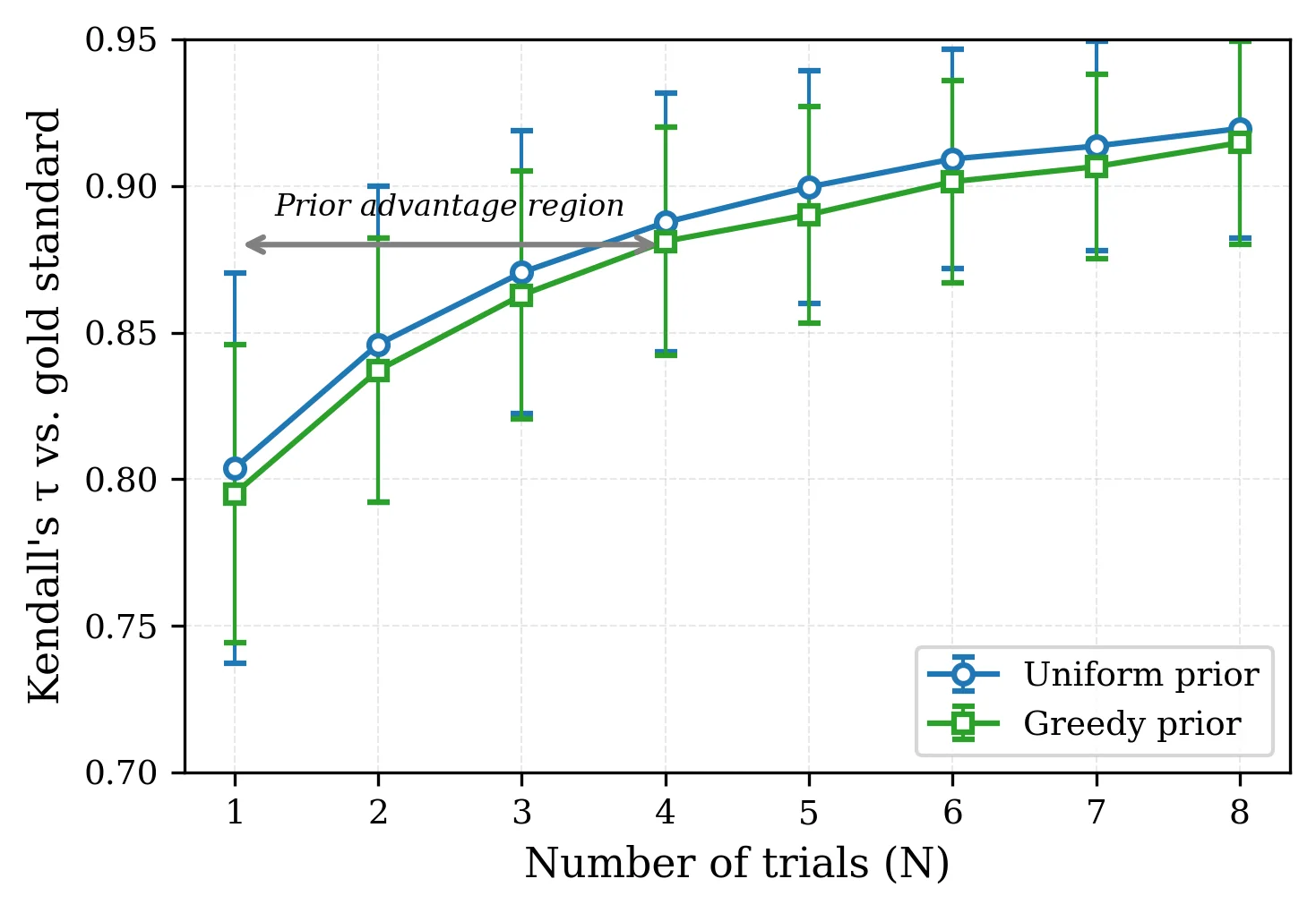
conservative = rank.bayes(R, R0=R0, quantile=0.05)

At N = 1, the greedy prior can reduce the standard deviation of agreement by 16% to 52%.
That variance reduction is useful only when greedy decoding tracks the same ordering as stochastic sampling.
Use quantile=0.05 when you want a conservative lower-bound ranking.

import numpy as np
from scorio import rank
 
# 0 = invalid, 1 = wrong, 2 = partial, 3 = correct
R_cat = np.random.randint(0, 4, size=(11, 120, 5))
w = np.array([0.0, 0.0, 0.5, 1.0])
 
scheme_ranks, scheme_scores = rank.bayes(
    R_cat,
    w=w,
    return_scores=True,
)
 
scheme_lcb = rank.bayes(R_cat, w=w, quantile=0.05)

Changing the ranking target is just a matter of changing labels and weights.
Signal-rich schemes can become more self-consistent than correctness-only ranking at N = 1.
That does not mean they stay closest to the correctness-based gold standard.

The primitive object is a response tensor, not a single accuracy number.
Each model-question pair can be sampled repeatedly, so rankings change as the trial budget grows.
Methods that look similar at full budget can behave very differently when only one or two trials are available.

1 Collect repeated trials per question
→
2 Apply one ranking family to the tensor
→
3 Use Bayes_U@80 as the shared gold standard
→
4 Measure agreement and convergence as N changes
→
5 Prefer rules that stay stable at low budget

Main distinction: high-budget consensus tells you what methods eventually agree on; low-budget stability tells you what you can trust in practice.

Bump charts showing how 72 ranking methods agree with Bayes_U at full budget on BrUMO and HMMT — Agreement between full-trial rankings and Bayes_U@80 on an easier benchmark and a harder benchmark.

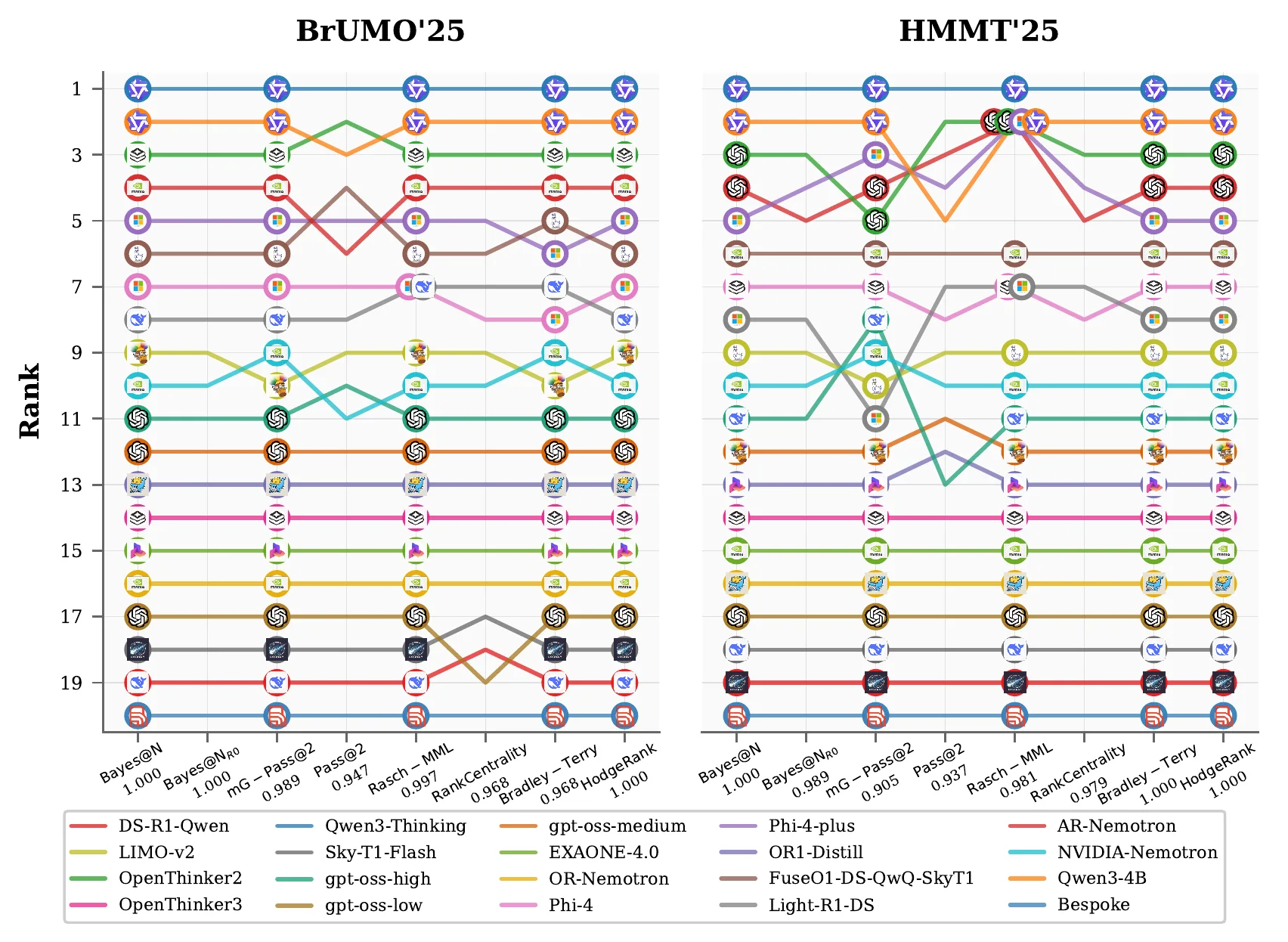
Across the four benchmarks, the mean Kendall τ_b versus Bayes_U@80 is 0.93 to 0.95.
Depending on the benchmark, 19 to 34 methods recover exactly the same full-trial ordering.
Divergence concentrates on harder benchmarks and a small set of voting or difficulty-weighted rules.

Agreement with the Bayes_U gold standard as the number of stochastic trials increases — Agreement improves as the trial budget grows, with the steepest gains in the first few trials.

The best methods reach τ_b ≈ 0.86 on the combined benchmark at a single trial.
Bayes_G@1 wins on AIME'24, AIME'25, and BrUMO'25, but not on HMMT'25 or the pooled benchmark.
High self-consistency does not imply closeness to the correctness-based gold standard.

Recommendation
Bayes_U@N is the safe default; add a greedy prior only after checking alignment.

Difference in gold-standard agreement between greedy and uniform priors across benchmarks — Greedy priors help on some easier or aligned benchmarks and hurt on the hardest or pooled settings.

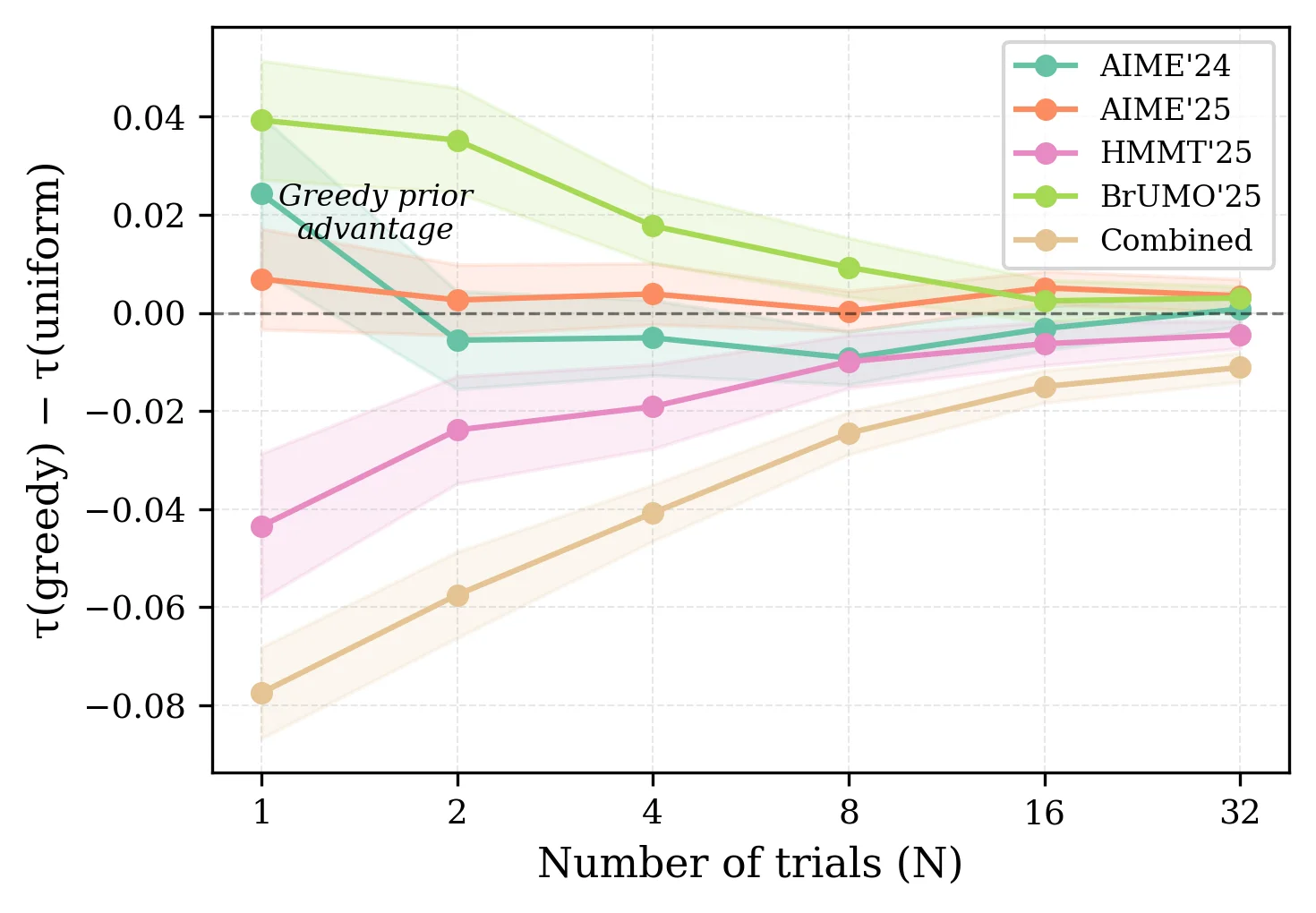
At N = 1, the greedy prior reduces the standard deviation of agreement by 16% to 52%.
The mean shift is positive on AIME'24, AIME'25, and BrUMO'25, but negative on HMMT'25 and Combined.
The advantage decays quickly as new stochastic evidence accumulates.

Rank-alignment diagnostics comparing greedy-decoding rankings with stochastic-sampling rankings — Greedy-sampling agreement is strongest on BrUMO and weakest on HMMT.

BrUMO is the easiest benchmark and shows the largest positive prior effect.
HMMT is harder, less aligned, and is the setting where Bayes_G@N hurts agreement with Bayes_U@80.
Difficulty and alignment move together: when greedy decoding ceases to be a faithful proxy, shrinkage becomes bias.

Scatter plot showing the tradeoff between agreement with the gold standard and self-consistency for categorical schemes — Schemes in the upper-left are stable but drift away from correctness; schemes in the lower-right stay closer to the gold standard.

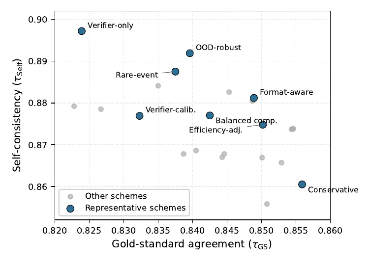
On the combined benchmark at N = 1, conservative ranking reaches τ_GS = 0.856 and τ_Self = 0.861.
Verifier-only ranking is more self-consistent at 0.897, but it drops to 0.824 against the gold standard.
Richer signals are useful when they reflect the real target, not when they are treated as a free upgrade to correctness-only ranking.

Takeaway
Categorical Bayes ranking is powerful, but the rubric has to be reported and justified.

ACL 2026 Main

Dense benchmark ranking under repeated sampling

Test-time scaling evaluates reasoning LLMs by drawing multiple outputs per prompt, but ranking methods in this regime have been compared much less systematically than model families. This paper fixes a correctness-based reference ranking, Bayes_U@80, then measures how closely alternative methods recover that ordering as the trial budget shrinks.

The main empirical result is two-part: full-budget agreement is high across most ranking families, but low-budget reliability is much less uniform. Bayes_U@N is the safest default, Bayes_G@N can help when greedy and sampling orderings are aligned, and categorical schemes must be treated as explicit target changes rather than free performance gains.

72 ranking methods 20 models x 4 benchmarks x up to 80 trials Bayes_U@N as the practical default

Response tensor

$$R \in \{0, 1, \ldots, C\}^{L \times M \times N}$$

Correctness-based reference

$$\text{Gold standard} = \mathrm{Bayes}_{\mathcal{U}}@80 \equiv \mathrm{avg}@80$$

Agreement metric

$$\tau_b\!\left(\text{method}@n,\ \mathrm{Bayes}_{\mathcal{U}}@80\right)$$

Input: repeated-trial tensor R
1. Choose a ranking family
2. Compute method@n at each budget n
3. Compare each ranking to Bayes_U@80
4. Average agreement across resamples
5. Prefer rules that stay close at small n

Pointwise methods operate directly on per-question solve rates or posterior summaries.
Pairwise, graph, and voting rules collapse the tensor into other comparison structures before ranking.
The paper separates correctness-based ranking from richer categorical targets instead of mixing them together.

Bump chart of method agreement with Bayes_U at N equals 80 across two representative benchmarks — Easier benchmarks keep most methods tightly clustered; harder benchmarks reveal where ranking families diverge.

Average Kendall τ_b with Bayes_U@80 ranges from 0.93 to 0.95 across benchmarks.
Between 19 and 34 methods recover exactly the same full-trial ordering, depending on the dataset.
The worst disagreements come from a small tail of voting rules and difficulty-weighted baselines rather than from the main Bayesian and pairwise families.
That high-budget consensus explains why the low-budget regime is the decisive comparison.

Detailed low-budget stability curves showing agreement as the number of trials increases — Agreement rises rapidly in the first few trials; most of the ranking uncertainty is concentrated at tiny N.

AIME'24 Bayes_G@1, τ_b = 0.779 +/- 0.034

AIME'25 Bayes_G@1, τ_b = 0.798 +/- 0.045

HMMT'25 Bayes_U@1 tie, τ_b = 0.790 +/- 0.053

BrUMO'25 Bayes_G@1, τ_b = 0.858 +/- 0.028

Combined Bayes_U@1 tie, τ_b = 0.865 +/- 0.049

Bayes_G@1 is the best method on the three better-aligned individual benchmarks.
On the hardest benchmark and on the pooled evaluation, the same shrinkage becomes a liability, so Bayes_U@1 stays in the tied best class.
The best self-consistent method is not always the method closest to the gold standard.

Prior-effect curves comparing Bayes_G and Bayes_U across benchmarks — The greedy prior cuts variance at tiny N everywhere, but the sign of the mean shift depends on alignment.

Interpretation
A prior is shrinkage toward the greedy ordering. Shrinkage helps only when that ordering is a faithful proxy for the stochastic ranking target.

Variance effect 16% to 52% standard-deviation reduction in τ_b at N = 1.

Best-case regime BrUMO: highest greedy-sampling alignment and strongest positive shift.

Failure regime HMMT and Combined: misalignment makes the prior bias the ranking away from Bayes_U@80.

Alignment is not an abstract diagnostic; it predicts the sign of the prior effect.
The empirical trend suggests a simple policy: run a pilot, measure greedy-sampling agreement, and only then decide whether to inject R0.

Tradeoff plot for categorical schemes at N equals 1 on the combined benchmark — Signal-rich schemes occupy the high-self-consistency corner, while conservative schemes stay closer to the correctness-based target.

Eight representative schemes were selected from a larger family spanning correctness, format, verifier, efficiency, OOD, and abstention signals.
Verifier-only and OOD-robust schemes are among the most self-consistent but also among the furthest from Bayes_U@80.
Correctness-driven schemes remain above τ_GS = 0.80 on the harder benchmarks, while verifier-heavy schemes degrade more sharply.
The right interpretation is target design: if the rubric matters, rank under that rubric and report it explicitly.

Practical rule
Do not describe categorical ranking as a free improvement over correctness-only evaluation. It is a different objective with different tradeoffs.

from scorio import rank
 
rank.avg(R)
rank.bayes(R, R0=None, quantile=None)
rank.pass_at_k(R, k=3)
rank.bradley_terry(R)
rank.pagerank(R)

Default Bayes_U@N for correctness-based leaderboards.

Add a prior Only after a pilot shows greedy and stochastic rankings are aligned.

Use categories When the rubric is the real task definition, not when you only want a more stable number.

The same API surface lets you swap ranking families without changing the evaluation tensor.
That makes the methodological comparison reproducible instead of embedding ranking choices in ad hoc scripts.

Ranking Reasoning LLMs under Test-Time Scaling

Setup

APIs

Ranking families

Empirical priors

Categorical ranking

Why ranking under test-time scaling is different

At N = 80, most reasonable methods agree

Most of the practical risk is at N = 1

Greedy priors reduce variance, but can also inject bias

Alignment explains when the prior helps

Categorical schemes trade off fidelity and self-consistency

Dense benchmark ranking under repeated sampling

Problem setup and evaluation protocol

Full-budget agreement is high but not uniform

Single-trial ranking separates the useful defaults from the brittle ones

Why the greedy prior helps some datasets and hurts others

Categorical ranking changes the target, not just the estimator

Scorio makes the comparison space explicit