Don't Pass@k: A Bayesian Framework for Large Language Model Evaluation

Paper digest + setup

Setup

Scorio starts from a results matrix R with M problems by N trials and turns evaluation into posterior inference over question-level outcome probabilities instead of an at-least-one-success surrogate like Pass@k.

The core move is to tally category counts per question, combine them with a Dirichlet prior, and return a closed-form posterior mean mu, uncertainty sigma, and optional credible bounds through one shared API.

The same pipeline covers binary correctness, rubric-weighted scoring, and prior transfer through R0; on AIME, HMMT, and BrUMO, this gives faster convergence and more stable rankings than Pass@k.

Why replace Pass@k? It tracks at least one success in k tries, which can reshuffle rankings when N is small.
What Bayes@N adds: exact posterior uncertainty, interval-aware decisions, and one inference layer for binary or categorical outcomes.
What stays simple: change labels in R, change weights in w, and optionally pass R0 when earlier evidence is justified.

Results Matrix R.shape == (M, N)

Rubric Weights w.shape == (C + 1,)

Prior Evidence R0.shape == (M, D)

Posterior Output (mu, sigma[, lo, hi])

Function	Returns	Description
`bayes(R, w=None, R0=None)`	`(μ, σ)`	Posterior mean and uncertainty for binary or categorical outcomes.
`bayes_ci(R, w=None, R0=None)`	`(μ, σ, lo, hi)`	Bayes@N with a credible interval.
`avg(R, w=None)`	`(a, σ_a)`	Average score with Bayesian uncertainty calibration.
`avg_ci(R, w=None)`	`(a, σ_a, lo, hi)`	Avg@N with a credible interval.
`pass_at_k(R, k)`	`p`	Pass@k estimate for binary outcomes.
`pass_at_k_ci(R, k)`	`(μ, σ, lo, hi)`	Pass@k with a credible interval.
`pass_hat_k(R, k)`	`p`	Pass^{^}k, the all-correct probability.
`g_pass_at_k_tau(R, k, tau)`	`p`	Generalized Pass@k with threshold `tau`.
`mg_pass_at_k(R, k)`	`p`	Mean generalized Pass@k across majority thresholds.

Companion *_ci variants return (mu, sigma, lo, hi).

import numpy as np
from scorio import eval
 
# Binary outcomes: 1 = correct, 0 = incorrect
R = np.array([
    [0, 1, 1, 0, 1],
    [1, 1, 0, 1, 1],
])
 
k = 3
tau = 2 / 3  # require at least 2 correct out of 3
 
mu, sigma, lo, hi = eval.bayes_ci(R, bounds=(0.0, 1.0))
print(f"Bayes@N: mu={mu:.6f}, sigma={sigma:.6f}, CI=[{lo:.6f}, {hi:.6f}]")
 
mu, sigma, lo, hi = eval.avg_ci(R, bounds=(0.0, 1.0))
print(f"Avg@N: mu={mu:.6f}, sigma={sigma:.6f}, CI=[{lo:.6f}, {hi:.6f}]")
 
mu, sigma, lo, hi = eval.pass_at_k_ci(R, k)
print(f"Pass@{k}: mu={mu:.6f}, sigma={sigma:.6f}, CI=[{lo:.6f}, {hi:.6f}]")
 
mu, sigma, lo, hi = eval.g_pass_at_k_tau_ci(R, k, tau)
print(f"G-Pass@{k} (tau={tau:.3f}): mu={mu:.6f}, sigma={sigma:.6f}, CI=[{lo:.6f}, {hi:.6f}]")
 
mu, sigma, lo, hi = eval.mg_pass_at_k_ci(R, k)
print(f"mG-Pass@{k}: mu={mu:.6f}, sigma={sigma:.6f}, CI=[{lo:.6f}, {hi:.6f}]")

bayes_ci, avg_ci, pass_at_k_ci, g_pass_at_k_tau_ci, and mg_pass_at_k_ci all return (mu, sigma, lo, hi).
The Pass interval calls are binary-only; use bayes_ci with rubric weights in categorical evaluation.

import numpy as np
from scorio import eval
 
# R: results from top-p sampling
R = np.array([
    [0, 1, 2, 2, 1],
    [1, 1, 0, 2, 2],
])
 
# R0: results from greedy sampling on the same questions
R0 = np.array([
    [2],
    [1],
])
 
w = np.array([0.0, 0.5, 1.0])
 
mu, sigma = eval.bayes(R, w)
print(f"Top-p only: mu={mu:.6f}, sigma={sigma:.6f}")
 
mu, sigma = eval.bayes(R, w, R0)
print(f"Top-p + greedy prior: mu={mu:.6f}, sigma={sigma:.6f}")
 
# Expected:
# Top-p only: mu=0.562500, sigma=0.091998
# Top-p + greedy prior: mu=0.583333, sigma=0.085165

Use R0 to reuse pilot data, earlier benchmarks, or related previous runs.
The results from one sampling strategy can serve as a prior for another.
The main evaluation call stays the same; the prior just becomes another input to the posterior.

import numpy as np
from scorio import eval
 
# 0 = incorrect, 1 = partial credit, 2 = correct
R = np.array([
    [0, 1, 2, 2, 1],
    [1, 1, 0, 2, 2],
])
 
w = np.array([0.0, 0.5, 1.0])
 
mu, sigma = eval.bayes(R, w)
print(f"Bayes@N: mu={mu:.6f}, sigma={sigma:.6f}")
 
# 0 = invalid, 1 = wrong-high-confidence, 2 = wrong-low-confidence, 3 = correct
R_conf = np.array([
    [3, 2, 3, 1, 3],
    [2, 3, 0, 3, 1],
])
w_conf = np.array([0.0, 0.0, 0.25, 1.0])
 
mu, sigma, lo, hi = eval.bayes_ci(R_conf, w_conf)
print(f"Confidence-aware: mu={mu:.6f}, sigma={sigma:.6f}, CI=[{lo:.6f}, {hi:.6f}]")
 
# Bayes@N: mu=0.562500, sigma=0.091998
# 95% CrI: [0.382188, 0.742812]
# Confidence-aware rubric: mu=0.444444, sigma=0.100539, CI=[0.247392, 0.641497]

This example uses three categories: incorrect, partial credit, and correct.
Changing the score semantics is just a matter of changing labels in R and weights in w.

Pass@k estimates the probability of at least one success in k tries, not a model's underlying success probability.
With limited samples, rankings can be unstable and sensitive to decoding and sampling noise.
It lacks a simple closed-form uncertainty estimate and does not naturally extend to partial-credit rubrics.

1 Run N samples per question
→
2 Score each attempt (binary/rubric)
→
3 Tally category counts
→
4 Dirichlet posterior over outcomes
→
5 Report μ, σ, and CIs

Bayes@N turns evaluation into posterior inference over question-level outcome probabilities.

Probability-mass and rank-trace plots comparing Bayes@N with pass@2, pass@4, and pass@8 across AIME24, AIME25, HMMT25, and BrUMO25. — Convergence@n PMFs compare Bayes@N with pass@2/4/8 across AIME24/25, HMMT25, and BrUMO25. Ranking traces show fast convergence on BrUMO25 and non-convergence on AIME25.

Convergence@n
PMFs compare Bayes@N with pass@2/4/8 across AIME'24/'25, HMMT'25, and BrUMO'25.

Ranking traces show fast convergence on BrUMO'25 and non-convergence on AIME'25.

Four benchmark plots showing Bayes@N and Pass variants across AIME24, AIME25, HMMT25, and BrUMO25 with Kendall tau rising faster for Bayes@N. — Bayes@N reaches high agreement with the gold-standard ranking quickly, while Pass@k variants require substantially more trials.

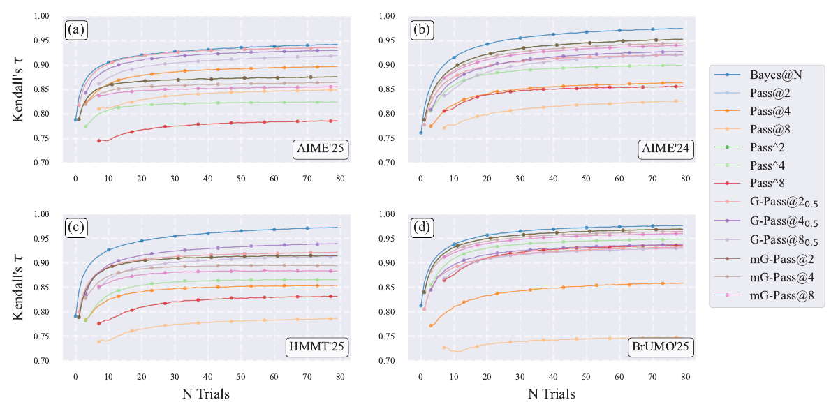
On AIME'24, AIME'25, HMMT'25, and BrUMO'25, Bayes@N reaches τ > 0.90 by N = 10 and tracks the gold-standard ranking much faster than Pass@k.
AIME'25 remains partially unresolved even at N = 80, showing why interval-aware reporting is necessary.

Posterior on question α:

$$\pi_{\alpha} \mid R_{\alpha} \sim \mathrm{Dir}\left(n^{0}_{\alpha 0} + n_{\alpha 0}, \ldots, n^{0}_{\alpha C} + n_{\alpha C}\right)$$

Weighted rubric metric:

$$\bar{\pi} = \frac{1}{M} \sum_{\alpha} \sum_{k} w_k \pi_{\alpha k}$$

Output both a posterior mean $\mu(R)$ and exact uncertainty $\sigma(R)$.
Binary evaluation is a special case; categorical rubrics use the same machinery.
Under a uniform prior in the binary case, Bayes@N has the same ordering as avg@N / Pass@1, but adds principled uncertainty.

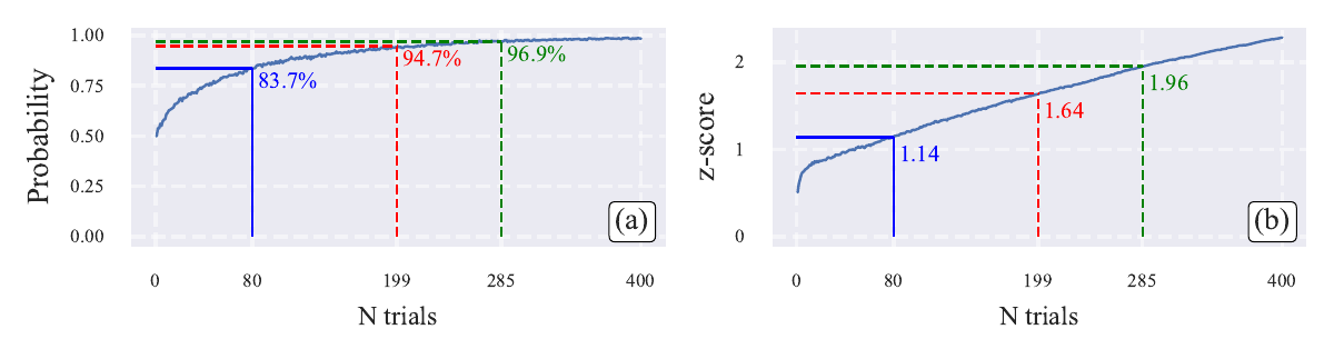
Illustrative Bayesian credible-interval plots showing how overlap determines whether a ranking is resolved. — Recommended protocol: sample N attempts, score each attempt with a binary or rubric-aware labeler, report Bayes@N with CIs, then extend N only if needed.

Practical rule
If credible intervals overlap, do not call a winner. For pairwise rankings, z = 1.645 implies 95% confidence in the ordering.

Recommended protocol: sample N attempts, score each attempt with a binary or rubric-aware labeler, report Bayes@N with credible intervals, then extend N only if needed.

Heatmaps showing convergence worsening as the number of compared models increases from 5 to 15. — Scaling model comparisons makes interval-aware stopping rules essential: strict point-estimate rankings become increasingly brittle as the leaderboard widens.

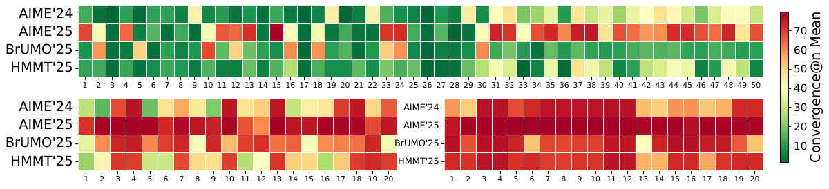
Mean convergence@n worsens as the number of compared models increases from 5 to 15.
Without credible intervals, many subsets fail to stabilize within 80 trials; scaling to 20 models makes the problem severe on all four datasets.
Posterior intervals provide a transparent stopping rule when strict point-estimate rankings are not yet trustworthy.

Categorical ranking plot showing how model positions change under different rubric schemas. — Ranking across categorical schemas remains interpretable because posterior means and uncertainty stay on the same footing.

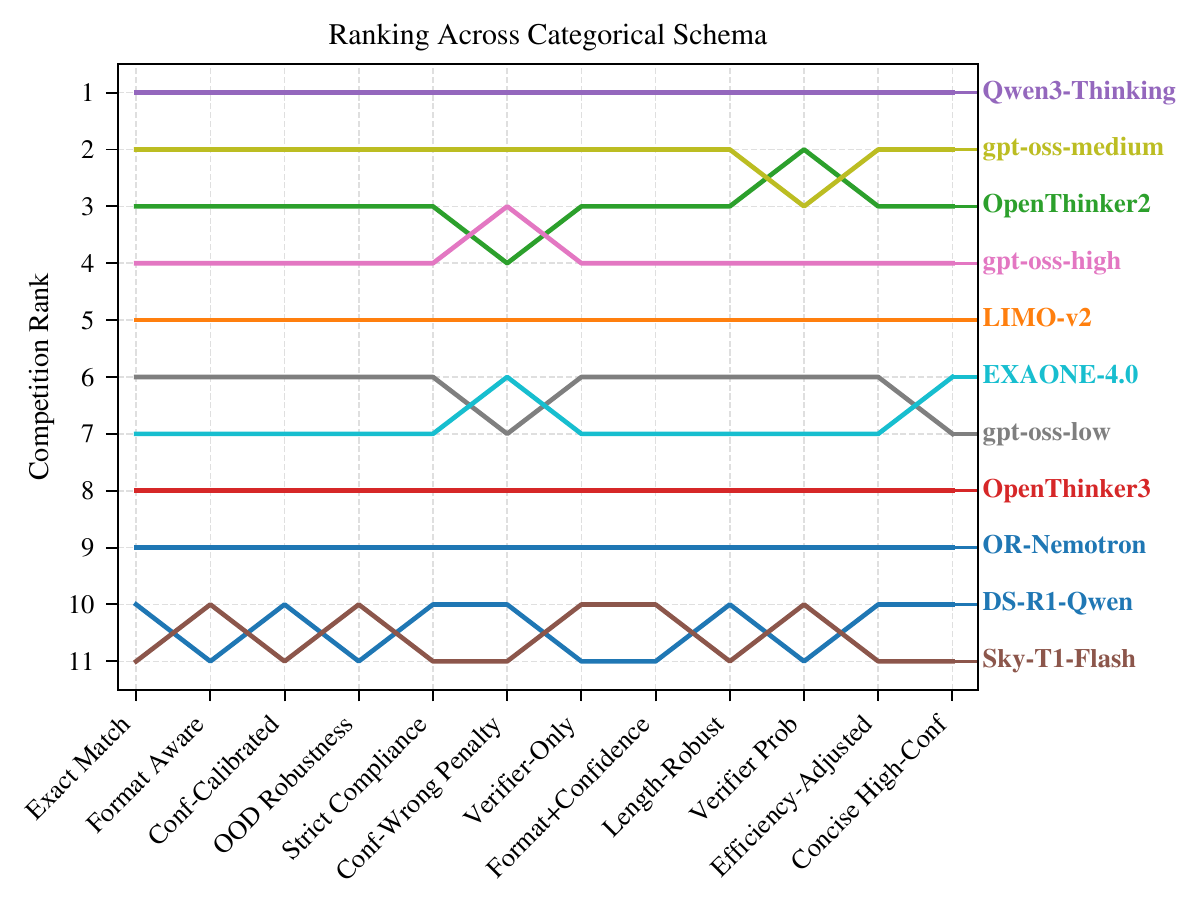
Treat outcomes as categorical: correct, partial credit, format errors, refusals, verifier signals, efficiency penalties, and more.
Different weight vectors encode different evaluation goals while keeping posterior uncertainty explicit.
Across schemas, Qwen3-Thinking remains first; rubric choice mainly reshuffles the middle of the pack.

Takeaway: replace Pass@k with Bayes@N + credible intervals for stable, uncertainty-aware ranking, and use categorical scoring beyond 0/1 correctness.

Acknowledgment: This research was supported in part by NSF awards 2117439, 2112606, & 2320952.

Bayes@N

Bayes@N as Dirichlet-multinomial posterior inference

Pass@k estimates the probability of at least one success in k tries, which is not the same as the latent per-question success distribution of a model. Bayes@N starts from an $M \times N$ result matrix $R_{\alpha i} \in \{0, \ldots, C\}$, places a Dirichlet prior on each question-level outcome vector $\pi_{\alpha}$, and evaluates the weighted target $\bar{\pi} = \frac{1}{M} \sum_{\alpha} \sum_{k} w_k \pi_{\alpha k}$. This turns evaluation into posterior inference over latent outcome probabilities rather than an at-least-one-success surrogate.

Because the posterior is conjugate, Bayes@N yields exact closed-form expressions for $\mu(R)$ and $\sigma(R)$, supports prior evidence through an optional $M \times D$ matrix $R^{0}$, and gives an operational stopping rule: rank by posterior mean, merge unresolved comparisons with credible intervals, and spend additional trials only where the z-score is still too small. The same construction covers binary correctness, partial-credit rubrics, format-sensitive scoring, verifier-based labels, and efficiency-aware penalties.

Exact closed-form $\mu$ and $\sigma$ 95% pairwise confidence: $z = 1.645$ Uniform prior: same ordering as avg@N

Run the model $N$ times on each of $M$ questions and record categorical labels $R_{\alpha i} \in \{0, \ldots, C\}$. For question $\alpha$, the latent probability simplex is $\pi_{\alpha} = (\pi_{\alpha 0}, \ldots, \pi_{\alpha C})$.

Weighted metric over latent outcome probabilities

$$\bar{\pi} = \frac{1}{M} \sum_{\alpha=1}^{M} \sum_{k=0}^{C} w_k \pi_{\alpha k}$$

Posterior for each question

$$\pi_{\alpha} \mid R_{\alpha} \sim \mathrm{Dir}(\nu_{\alpha 0}, \ldots, \nu_{\alpha C}), \quad \nu_{\alpha k} = n_{\alpha k} + n^{0}_{\alpha k}$$

Uniform or informative prior counts

$$n^{0}_{\alpha k} = 1 + \sum_{i=1}^{D} \delta_{k, R^{0}_{\alpha i}}, \qquad T = 1 + C + D + N$$

Binary correctness is the special case $C = 1$ with weights $[0, 1]$.
Categorical scoring simply changes the labels and the weight vector w; the inference machinery is unchanged.
The optional prior matrix $R^{0}$ makes prior evidence explicit rather than hidden in a heuristic.

Posterior mean

$$\mu = w_0 + \frac{1}{MT} \sum_{\alpha=1}^{M} \sum_{j=0}^{C} \nu_{\alpha j}(w_j - w_0)$$

Posterior variance

$$\sigma^{2} = \frac{1}{M^{2}(T + 1)} \sum_{\alpha=1}^{M} \left\{ \sum_{j=0}^{C} \left(\frac{\nu_{\alpha j}}{T}\right)(w_j - w_0)^{2} - \left[\sum_{j=0}^{C} \left(\frac{\nu_{\alpha j}}{T}\right)(w_j - w_0)\right]^{2} \right\}$$

Uniform-prior relationship to avg@N

$$\mu = A + \frac{N}{1 + C + N} a$$

Under a uniform prior, Bayes@N and avg@N induce exactly the same ordering, but Bayes@N also outputs exact uncertainty.
The formulas are valid at finite M and N; they do not rely on CLT, Wald intervals, or asymptotic normality.
For small benchmarks, this avoids the interval pathologies that appear when uncertainty is approximated too aggressively.

EvaluatePerformance(R, [R0], w):
  T = 1 + C + D + N
  for alpha in 1..M:
    for k in 0..C:
      n_alpha_k  = sum_i delta(k, R_alpha_i)
      n0_alpha_k = 1 + sum_i delta(k, R0_alpha_i)
      nu_alpha_k = n_alpha_k + n0_alpha_k
  mu = w0 + (1 / MT) sum_alpha sum_j nu_alpha_j (w_j - w0)
  sigma = sqrt(closed-form variance on nu / T)
  return mu, sigma

Closed Form Tally counts, then plug into closed form

No iterative optimization, sampling-based posterior estimation, or bootstrap is required to compute μ and σ.
The only state the evaluator needs is the count table per question and category.
This is why Bayes@N is practical even when the benchmarking budget is dominated by model inference rather than post-processing.

The paper uses Bayes@80, equivalently avg@80, as the practical gold-standard ranking for finite-budget experiments.
Across AIME'24, AIME'25, HMMT'25, and BrUMO'25, Bayes@N reaches Kendall τ > 0.90 by N = 10; only AIME'25 remains below full convergence at N = 80.
Mean convergence@n is about 44.2 on HMMT and 27.1 on BrUMO for Bayes@N, versus roughly 69.5 and 48.5 for the best Pass@k alternatives.
Worst-case bootstrap trajectories still need N = 75 on AIME'24, N = 78 on HMMT, N = 68 on BrUMO, and do not converge within 80 trials on AIME'25.

Pairwise ranking confidence

$$z = \frac{|\mu - \mu'|}{\sqrt{\sigma^{2} + (\sigma')^{2}}}, \qquad \rho = \frac{1}{2}\left(1 + \operatorname{erf}\left(\frac{z}{\sqrt{2}}\right)\right)$$

N = 80 $z \asymp 1.14$, $\rho = 83.7\%$

N = 199 $z = 1.645$, $\rho = 95\%$

N = 285 $z = 1.96$, $\rho = 96.9\%$

Illustrative credible-interval plots used for the Bayes at N decision rule. — If intervals overlap, keep the comparison unresolved and allocate more trials only where needed.

The biased-coin experiment shows why a strict rank ordering at N = 80 can be overconfident: some adjacent gaps are still statistically unresolved.
At the benchmark level, AIME'25 has the most compressed Bayes@80 ranking with credible intervals, signaling that additional trials are required.

Format Aware schema

1: wrong ∧ unboxed 2: wrong ∧ boxed 3: correct ∧ unboxed 4: correct ∧ boxed

Twelve categorical schemata in the paper combine correctness, boxing, confidence, verifier signals, OOD behavior, and efficiency into a unified posterior framework.
Across selected schemata, Qwen3-Thinking remains first, while rubric choice mostly changes the middle ranks.
Several schema families agree closely at the top and bottom of the leaderboard, with most movement concentrated in the middle ranks.
Bayes@N quantifies finite-sample uncertainty in the chosen rubric; it does not fix benchmark bias or bad rubric design, so schemas must be reported explicitly.

Takeaway
Bayes@N is a single inference layer for binary accuracy, graded rubrics, and interval-aware ranking.

Three-panel plot showing a Kendall tau histogram for original versus updated synthetic models, Kendall tau versus trial count under uniform and non-uniform priors, and delta tau relative to the uniform prior. — Panel (a) shows the original and updated synthetic rankings are correlated but usually not identical; panels (b) and (c) show that small D helps early, while large D eventually hurts.

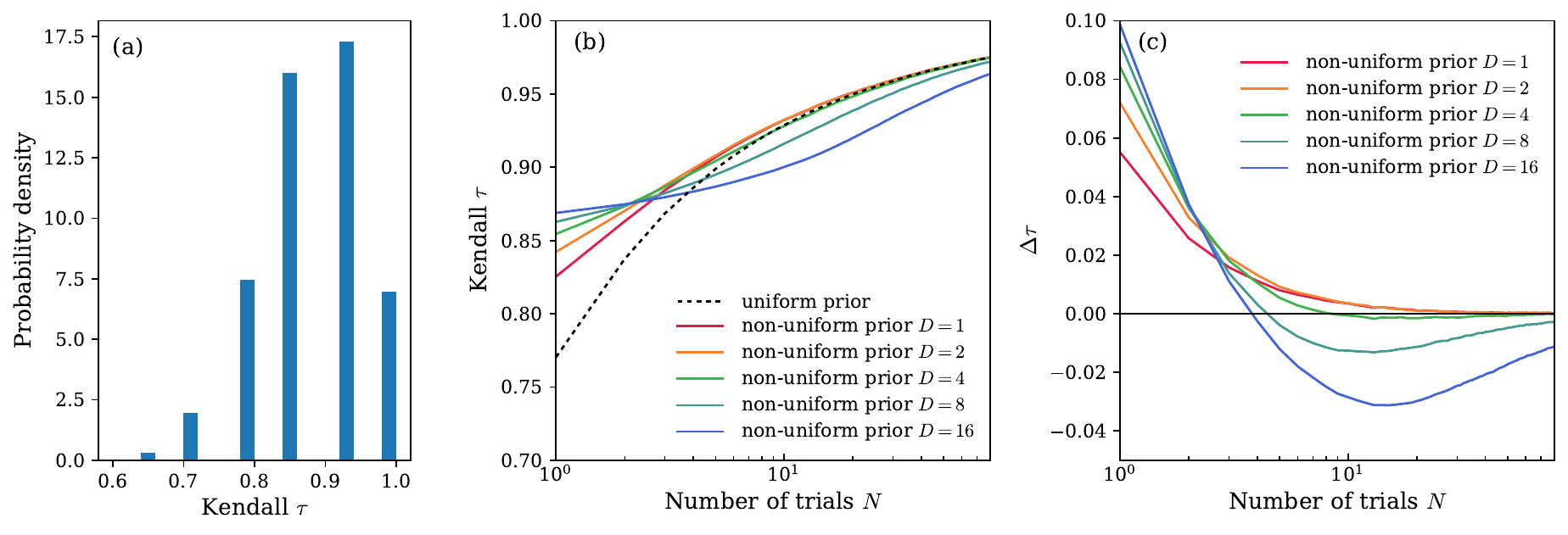
Takeaway
Non-uniform priors can accelerate convergence when the old and new rankings are correlated, but D must be chosen judiciously and reported explicitly.

Setup Eight synthetic "updated" models are ranked using priors derived from their correlated original versions.

Benefit At low trial counts, non-uniform priors with D = 1, 2, or 4 raise Kendall τ above the uniform-prior baseline.

Failure Mode With D = 8 or 16, the prior can dominate for too long and push Δτ below zero at larger N.

Panel (a): over 50k updates, old and new rankings have mean Kendall τ ≈ 0.88.
Panel (b): at low N, modest priors beat the uniform prior.
Best early gains come from small prior depth: D = 1, 2, or 4.
Panel (c): large D eventually hurts by overpowering new evidence.

Don't Pass@k: A Bayesian Framework for Large Language Model Evaluation

Setup

APIs

Credible interval

Prior knowledge

Categorical evaluation

Why replace Pass@k?

Convergence and Rank Stability

Benchmarks: rankings with fewer trials

Bayesian estimator and the decision rule

Leaderboard grows -> interval-aware evaluation matters more

Beyond binary correctness: rubric-aware Bayes@N

Bayes@N as Dirichlet-multinomial posterior inference

Problem setup and posterior construction

Closed-form estimator, uncertainty, and avg@N equivalence

Algorithm

Convergence to the gold ranking

Decision rule and confidence

Categorical rubrics

Potential benefits of non-uniform priors