Simulating LLM Answers to Evaluation Datasets

TL;DR: Evaluating LLMs is tricky because these models are probabilistic and their outputs vary across runs, especially in the case of reasoning models. Simulation helps us understand this variability and stress-test our evaluation or ranking methods.

We can model LLM responses as flipping biased coins. A simple Bernoulli model captures basic success/failure patterns. Adding Beta distributions lets us represent question-to-question variation in difficulty. Item Response Theory provides an even richer framework that explicitly models model ability, question difficulty, discrimination, and guessing.

By simulating complete evaluation datasets (multiple models, multiple questions, multiple runs), we can test whether our metrics are robust, compute meaningful confidence intervals, and determine how many runs we really need for reliable rankings. For a real application of simulation, check out Don’t Pass@𝑘: A Bayesian Framework for Large Language Model Evaluation.

The Coin Flip Analogy

Let's start by one model trying to solve a problem multiple times. Each attempt either succeeds (heads) or fails (tails). If the model has some fixed probability of success (i.e., model's ability for perfomance), this looks like flipping a biased coin.

Single Coin, Many Flips

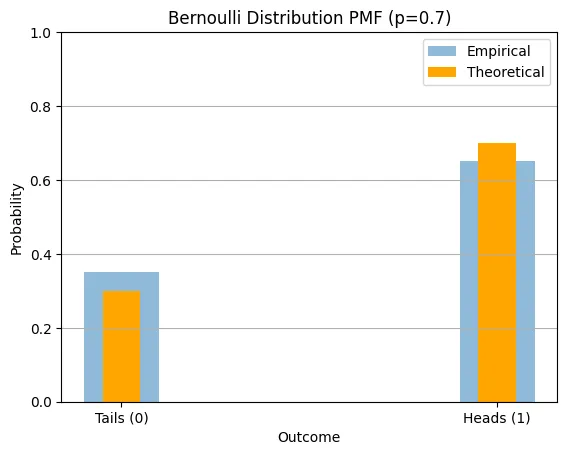
The simplest case can be modeled via a Bernoulli distribution. Let's say our coin has a 70% chance of landing heads. Mathematically, if $X$ represents a single flip, then:

$P(X = 1) = p = 0.7$ $P(X = 0) = 1 - p = 0.3$

where 1 represents heads (success) and 0 represents tails (failure).

Now, if we flip this coin 80 times, we're drawing 80 independent samples from this distribution. The theoretical distribution is fixed (70% heads, 30% tails), but our empirical results will vary slightly due to randomness. With 80 flips, we might observe something like 72% heads or 68% heads. The gap between theoretical and empirical values shrinks as we increase the number of flips. This captures a fundamental truth about LLM evaluation: even if a model has a true underlying success rate, any finite sample of runs will show some variation around that rate. Note that in case of LLM evaluation, number of independent samples are limited to 8 or 16 due to cost constraints.

alt text

Many Coins, Many Flips

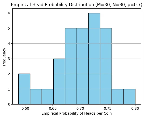
Now, let's suppose instead of one question, we have an evaluation dataset which can be represented as 30 different coins, and we flip each one 80 times (representing 80 runs per question). Each coin still has the same bias (70% heads), but now we're observing 30 parallel experiments. For each coin $i$ , we can compute its empirical success rate:

\hat{p}_i = \frac{1}{N}\sum_{j=1}^{N} X_{ij}

where $N = 80$ is the number of flips per coin and $X_{ij}$ is the outcome of the $j$ -th flip of coin $i$ .

When we look at the distribution of these 30 empirical rates, we see something interesting: they cluster around 0.7, but with some spread. Some coins might show 0.68, others 0.72, purely due to sampling variability. The overall average across all 2,400 flips (30 coins × 80 flips) will be very close to 0.7, but individual coins show variation.

This shows how different questions in an evaluation dataset might show different observed success rates for a model, even if the model's true capability is uniform.

alt text

Adding Question Difficulty

But here's where it gets more realistic. What if different questions have different difficulty levels? Not all problems are created equal.

We can model this with a Beta-Bernoulli setup. Instead of every coin having exactly 70% bias, we draw each coin's bias from a Beta distribution. The Beta distribution is perfect for this because it's defined on the interval (0, 1) and can take many different shapes depending on its parameters $\alpha$ and $\beta$ .

For a Beta distribution with parameters $\alpha = 7$ and $\beta = 3$ :

p \sim \text{Beta}(\alpha, \beta)

The mean is $\frac{\alpha}{\alpha + \beta} = \frac{7}{10} = 0.7$ , but individual draws will vary around this mean. Once we draw a specific $p$ value for a question, we then flip that question's coin using $p$ as the success probability.

This two-stage process captures an important aspect of real evaluation: questions vary in difficulty, and this variation adds another layer of uncertainty to our measurements.

We can go even further with a Beta mixture of Bernoullis. Here, for each of 80 runs, we draw a fresh probability $p_j$ from our Beta distribution and then perform one Bernoulli trial with that probability. This models a scenario where not only do questions vary, but each individual run has its own slight variations in conditions.

Mathematically, for run $j$ :

p_j \sim \text{Beta}(\alpha, \beta), X_j \sim \text{Bernoulli}(p_j)

This adds even more variability to our simulation, better capturing the complex, multi-layered uncertainty in real LLM evaluations.

Item Response Theory: A Richer Framework

While coin flips give us intuition, Item Response Theory (IRT) offers a framework that models both a model’s capability and the characteristics of each question.

In IRT, we model the probability of success using a few key parameters: ability $\theta$ (how capable the model is), difficulty $b$ (how hard the question is), discrimination $a$ (how well the question differentiates between strong and weak models), and sometimes guessing parameters.

The Rasch model (1-parameter logistic or 1PL model) is the simplest. It uses the logistic function $\sigma(x) = \frac{1}{1 + e^{-x}}$ to map the difference between ability and difficulty to a probability:

P(Y = 1 \mid \theta, b) = \sigma(\theta - b) = \frac{1}{1 + e^{-(\theta - b)}}

If a model's ability $\theta$ equals the question's difficulty $b$ , the success probability is exactly 0.5. As ability increases relative to difficulty, the probability approaches 1.

The 2-parameter logistic (2PL) model adds a discrimination parameter $a$ that controls how steeply the probability changes:

P(Y = 1 \mid \theta, b, a) = \sigma\big(a(\theta - b)\big) = \frac{1}{1 + e^{-a(\theta - b)}}

A larger $a$ means the item discriminates more sharply between models with abilities just below and just above the difficulty threshold.

The 3-parameter logistic (3PL) model acknowledges that sometimes models can guess correctly, adding a lower asymptote $c$ :

P(Y = 1 \mid \theta, b, a, c) = c + (1 - c) \cdot \sigma\big(a(\theta - b)\big)

Even a very weak model (low $\theta$ ) has at least probability $c$ of succeeding, perhaps by guessing or exploiting patterns.

The 4-parameter logistic (4PL) model adds an upper asymptote $d$ , recognizing that even very capable models might not achieve perfect success on some items:

P(Y = 1 \mid \theta, b, a, c, d) = c + (d - c) \cdot \sigma\big(a(\theta - b)\big)

Finally, for tasks with rubric scores or ordinal outcomes (not just pass/fail), Samejima's Graded Response Model extends IRT to ordered categories. With thresholds $b_1 < b_2 < \cdots < b_C$ and a common discrimination $a$ , the probability of scoring at or above category $k$ is:

P(Y \geq k \mid \theta, a, b_k) = \sigma\big(a(\theta - b_k)\big)

The probability of scoring exactly in category $k$ is then:

P(Y = k) = P(Y \geq k) - P(Y \geq k+1)

These IRT models are rooted in psychometrics and give us a principled way to generate synthetic evaluation data that capture realistic patterns of model performance and question characteristics. If you're curious about how IRT can be applied to LLMs, check out Simulating LLM Evaluation Datasets Using Psychometric Models.

Simulating LLM Evaluation Datasets

Now let's put it all together and simulate a complete evaluation scenario. Let's assume there are:

$L = 20$ models, ranging from weakest to strongest
$M = 30$ questions in our evaluation dataset
$N = 80$ runs per question (to account for stochastic sampling)

We want to generate synthetic success/failure outcomes for all combinations: a three-dimensional array of size $L \times M \times N$ .

Generating Model Capabilities

First, we need to assign capability levels to our 20 models. We want them to span from relatively weak (say, 35% average success rate) to relatively strong (85% average success rate).

We could space them linearly:

$\theta_\ell = 0.35 + (0.85 - 0.35) \cdot \frac{\ell - 1}{L - 1} \quad \text{for } \ell = 1, \ldots, L$

But in practice, model capabilities often follow a more sigmoidal curve. We can map from a linear scale in "latent ability" space to success probability space using the logistic function:

$z_\ell = -2 + 4 \cdot \frac{\ell - 1}{L - 1}$ $\theta_\ell = 0.35 + (0.85 - 0.35) \cdot \sigma(z_\ell)$

This gives us a curved ladder where improvements are harder to achieve at the extremes and easier in the middle range, which often matches reality.

Adding Question-Level Variation

Each model has an average capability $\theta_\ell$ , but performance varies across questions. We can model this variation in two ways, depending on whether we want to use Beta-Bernoulli or IRT-based simulation.

Beta-Bernoulli approach: For model $\ell$ with mean capability $\theta_\ell$ , we draw each question's success probability from a Beta distribution. We convert the mean $\mu = \theta_\ell$ and a concentration parameter into Beta shape parameters:

\alpha_\ell = \mu \cdot \kappa, \beta_\ell = (1 - \mu) \cdot \kappa

where $\kappa$ (the concentration) controls how tightly questions cluster around the mean. A larger $\kappa$ means less question-to-question variation.

For each question $m$ and model $\ell$ , we draw:

p_{\ell m} \sim \text{Beta}(\alpha_\ell, \beta_\ell)

IRT-based approach: Alternatively, we can work in logit space. We convert the mean capability to logits, add Gaussian noise representing question variation, then map back to probability:

\text{logit}(\theta_\ell) = \log\left(\frac{\theta_\ell}{1 - \theta_\ell}\right), \text{logit}(p_{\ell m}) \sim \mathcal{N}(\text{logit}(\theta_\ell), \sigma^2)

p_{\ell m} = \sigma(\text{logit}(p_{\ell m})) = \frac{1}{1 + e^{-\text{logit}(p_{\ell m})}}

The parameter $\sigma$ controls the spread of question difficulties in logit space. Working in logit space is natural because it treats the probability scale symmetrically (equally spaced logits near 0.5 produce closer probabilities than equally spaced logits near 0 or 1).

Simulating Runs

Finally, for each model, each question, and each of the 80 runs, we flip a Bernoulli coin with the appropriate success probability:

X_{\ell m n} \sim \text{Bernoulli}(p_{\ell m})

where $X_{\ell m n} \in \{0, 1\}$ indicates whether model $\ell$ succeeded on question $m$ during run $n$ .

The result is a three-dimensional array of outcomes: $L \times M \times N = 20 \times 30 \times 80 = 48,000$ binary outcomes representing our simulated evaluation data.

What Can We Do With This?

Once we have this simulated dataset, we can test all sorts of things:

Metric robustness: Calculate Pass@k, average@N, or any other metric on this data and see how stable the estimates are. Does Pass@10 give us a reliable ranking of our 20 models? How much does it vary if we use a different random seed?
Sample size requirements: What happens if we only have 10 runs per question instead of 80? How much does our metric's variance increase? This helps us design efficient evaluation protocols.
Ranking stability: If we rank models by their metrics, how often does the ranking change when we resample? Are the top-3 models reliably in the top tier, or is there significant uncertainty?
Confidence intervals: We know the true model capabilities (we generated them!), so we can see how often our estimated confidence intervals contain the true values. This helps calibrate our uncertainty estimates.
Comparing evaluation protocols: We could simulate one dataset with 80 runs per question and another with 20 questions but 160 runs each. Which allocation of resources gives us better model discrimination?

The key insight is that simulation gives us ground truth. In real evaluation, we never know if Model A is truly better than Model B or if we just got lucky with our sample. In simulation, we know the answer, so we can audit whether our methods are giving us the right answers.

Interactive Simulation: Flip Your Own Coins

Below is an interactive module where you we set $L$ (number of models), $M$ (number of questions), and $N$ (samples per question), then simulate the coin-flip process. Each model has a different "true" success rate (the coin's bias), and we'll see how the estimated rankings stabilize—or don't—as you increase $N$ . Try starting with $N=1$ and watch the rankings jump around. Then crank it up to $N=20$ and see the variance collapse.

Conclusion

When we're evaluating large language models, we're working in a world of uncertainty. Models give different answers on different runs. Questions vary in difficulty. Metrics are just estimates with their own sampling error. All of this makes it surprisingly hard to answer simple questions like "Which model is better?"

Simulation doesn't eliminate this uncertainty, but it lets us quantify and understand it. By generating synthetic evaluation data where we control the ground truth, we can verify that our metrics and ranking methods actually work. We can determine how many samples we need. We can calculate confidence intervals that actually mean something.

Whether we're using simple Bernoulli models, Beta-Bernoulli hierarchies, or IRT frameworks, the core idea is the same: create a simplified world where we know the truth, then check if our methods can find it. If they can't find truth in our simplified simulations, they certainly won't find it in messy reality.