Ranking Reasoning LLMs under Test-Time Scaling
TL;DR: Test-time scaling samples a reasoning model many times per question, so a leaderboard is no longer one score per model but a stack of outcomes, one per model–question–trial. We turned that stack into a response tensor and asked which of the many ways to rank models you should trust. Across models and four Olympiad-style math benchmarks at trials, ranking methods, spanning , Bradley–Terry, Elo, IRT, voting rules, and PageRank, mostly agree: mean Kendall's with the accuracy-based gold standard is –, and – of them reproduce the exact same order. The choice of method only starts to matter when the budget collapses to a single trial. There, a greedy-decode prior () cuts ranking variance by –, but biases the order when greedy and sampled decoding disagree. All of it ships in scorio.
The question left over from Bayes@N
The previous paper settled a scoring question: replace Pass@ with a posterior estimate, , and you get stable numbers and honest uncertainty from far fewer samples. But a score is not a leaderboard. The moment we had the full dataset in hand ( reasoning models, four benchmarks, stochastic trials for every model–question pair), the open question changed shape. It was no longer "how do I score one model?" It was "how do I order twenty of them, and does it even matter which method I use?"
That question has an embarrassing number of answers. Statistics has been ranking things for two centuries: Bradley–Terry and Elo for head-to-head games, Borda and Copeland for votes, PageRank and HodgeRank for graphs, item response theory for tests. Each was designed for a different world, and each will happily produce a leaderboard from the same data. I expected them to disagree, and to spend the paper arguing about which one is right.
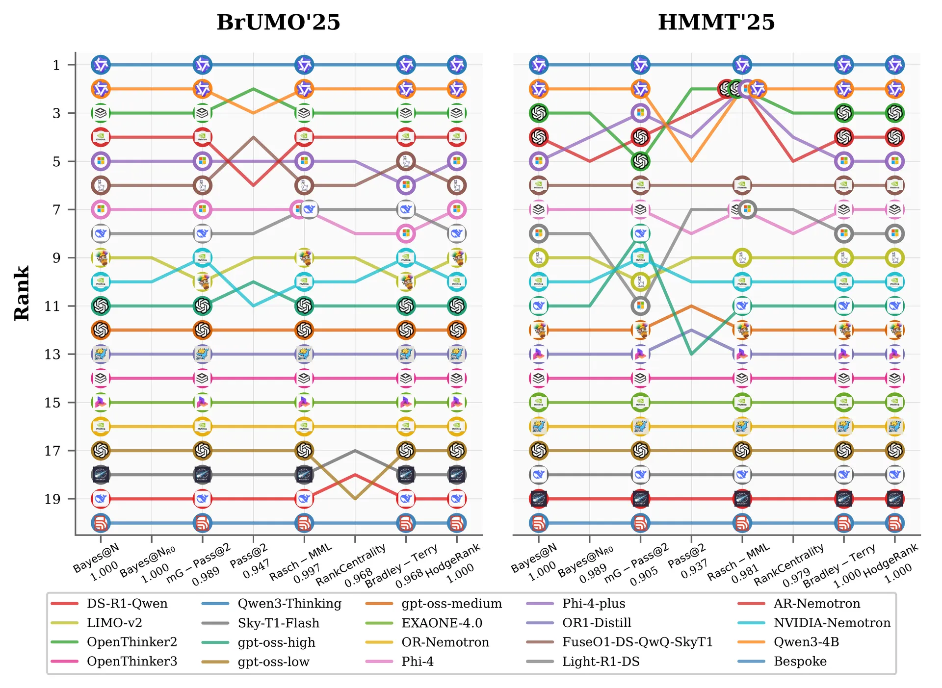
They mostly don't disagree. When you feed all trials to different ranking methods, the orderings pile up on top of each other. On the easier benchmark, several methods land on exactly the same order (the left panel of the figure above). The interesting behavior is not at full budget. It shows up when you can only afford one trial per question, which is exactly the regime a lab actually lives in.
Use it in practice
scorio installs with pip install scorio. It scores an outcome matrix (the Bayes@N side) and, new here, ranks models directly from a response tensor. Every ranking method takes the same tensor of shape (L, M, N) and returns a -indexed ranking where lower is better.
import numpy as np
from scorio import rank

# Response tensor: L=20 models, M=30 questions, N=80 trials, entries in {0, 1}
R = np.load("responses.npy")            # shape (20, 30, 80)

# Accuracy-based ranking (the gold-standard target)
ranking = rank.avg(R)

# Bayesian posterior-mean ranking (order-equivalent to avg@N under a uniform prior)
ranking, scores = rank.bayes(R, return_scores=True)
Swapping the method is a one-liner, which is what makes comparing them cheap:
| Function | Family | What it computes |
|---|---|---|
rank.avg(R) | pointwise | Mean-accuracy ranking (the gold-standard target) |
rank.bayes(R, R0=…, w=…, quantile=…) | Bayesian metric | Posterior-mean or lower-bound ranking; optional greedy prior and categorical weights |
rank.bradley_terry(R) | paired-comparison | Latent-strength ranking from pairwise win counts |
rank.elo(R) / rank.trueskill(R) | rating | Sequential / Bayesian rating over the induced match stream |
rank.borda(R) / rank.copeland(R) | voting | Treat each question as a voter and aggregate |
rank.pagerank(R) / rank.hodge_rank(R) | graph / spectral | Rank from the pairwise comparison graph |
rank.rasch_mml_credible(R) | IRT | Latent-ability estimate with a conservative posterior bound |
from scorio import rank, utils

gold = rank.bayes(R)     # Bayes_U@80, the accuracy-based reference
methods = {
    "avg":           rank.avg(R),
    "bradley_terry": rank.bradley_terry(R),
    "borda":         rank.borda(R),
    "pagerank":      rank.pagerank(R),
    "rasch_mml":     rank.rasch_mml_credible(R),
}
for name, r in methods.items():
    tau = utils.compare_rankings(r, gold)   # rank agreement (Kendall's tau_b)
    print(f"{name:14s} tau_b = {tau:.3f}")
A benchmark is a tensor, and every ranking method is a projection of it
Under test-time scaling, a benchmark stops being a table of one score per model. Every model–question pair is attempted times, so the raw evidence is a three-dimensional grid: model, question, trial, each cell a if that attempt was correct. Call it the response tensor. A single-run benchmark is just the slice of it.
Once you see the data this way, the zoo of ranking methods becomes less intimidating. They are not competing theories of the world; they are different ways of flattening the same tensor. Average accuracy and IRT read it pointwise, as a per-question solve rate. Bradley–Terry, Elo, and the voting rules read it pairwise, as counts of which model beat which. Plackett–Luce reads it setwise, as the set of models that solved each question–trial. What a method keeps or throws away in that flattening step is the whole story of why two leaderboards can differ.
Let index models and questions, with i.i.d. trials each. We observe binary outcomes
where if model solves question on trial . The natural pointwise summary is the per-question solve rate and its mean,
Because there is no universal ground truth for ranking methods, we score them against two targets. The first is an accuracy-based gold standard: the full-budget ordering , the Bayesian posterior mean with a uniform prior over all trials, which is order-equivalent to and allows ties. The second is a self-consistency target: the method's own full-trial ordering, method@80, which asks whether a method computed from one trial already agrees with the same method computed from eighty. Agreement is measured with Kendall's (tie-aware), so means an identical order.
The three representations
Every method we study consumes but operates on a projection of it.
Pointwise (model–question). Methods work on the matrix or its row means. Mean accuracy, inverse-difficulty weighting, and IRT-style models live here; when the trial axis is a stack of repeated Bernoulli observations with sufficient statistic , giving a binomial-response model. Evaluation metrics such as Pass@ and additionally use the per-question trial multiset before averaging over questions.
Pairwise (win / tie). For an ordered pair define
so that for every . In our fully-observed setting the comparison graph is complete, unlike Chatbot Arena, where the graph is sparse and evolving. Bradley–Terry and its tie extensions, Borda and Copeland, and graph/spectral methods (PageRank, Rank Centrality, HodgeRank, Nash averaging) all consume , typically via the tied-split win rate . Elo and TrueSkill instead replay the underlying stream of question–trial "matches."
Setwise (winner sets). For each question–trial the winner set ties above its complement. Plackett–Luce and Davidson–Luce operate on the collection , discarding the all-solved and none-solved events that carry no ranking information.
A consequence worth stating plainly: even as or grows, these methods need not converge to a single limiting order. Probabilistic paired-comparison models can emphasize different aspects of performance than an expected-accuracy metric, which is why "compute more trials" does not by itself make the choice of ranking method moot.
With 80 trials, the ranking method barely matters
This is the reassuring half of the result, and the one I did not expect. When every method gets the full , they agree with the accuracy-based gold standard, and largely with each other. The mean Kendall's between and the other methods is – per benchmark, the median is –, and a large block of methods reproduces the exact same ordering.
| Benchmark | Mean | Median | Min | #() | #() |
|---|---|---|---|---|---|
| AIME'24 | 0.941 | 0.989 | 0.682 | 20 | 40 |
| AIME'25 | 0.934 | 0.947 | 0.771 | 19 | 29 |
| HMMT'25 | 0.950 | 0.989 | 0.758 | 34 | 44 |
| BrUMO'25 | 0.954 | 0.968 | 0.789 | 26 | 49 |
| Combined | 0.962 | 0.989 | 0.748 | 22 | 53 |
Statistics are over the other methods, all computed from the full trials. The stragglers are a handful of voting rules (minimax and Nanson variants) and difficulty-weighted baselines.
The takeaway is a default: if you can afford a large trial budget, pick the simple, interpretable option. is exactly average accuracy in ranking terms, plus uncertainty for free. The exotic machinery neither helps nor hurts once the data is plentiful.
The choice only bites at one trial
Cut the budget to a single trial per question and the methods separate. We subsample one of the trials, recompute every ranking, repeat over all single-trial draws, and report the mean its standard deviation. (Pass@ needs at least two trials, so methods remain at .) Now the best method depends on which target you name: agreement with the accuracy gold standard, or self-consistency with a method's own full-budget order.
| Benchmark | Best vs. gold standard | Best self-consistency | ||
|---|---|---|---|---|
| AIME'24 | Rasch MML (LCB) | |||
| AIME'25 | Rasch MML (LCB) | |||
| HMMT'25 | (+20 tied) | Rasch MML (LCB) | ||
| BrUMO'25 | ||||
| Combined | (+20 tied) | Nanson (avg ties) |
Two things stand out. First, high self-consistency does not imply closeness to the accuracy order: Nanson's rule is the most repeatable method on the combined benchmark () yet trails badly on gold-standard agreement (). A method can converge cleanly to its own answer while that answer drifts away from accuracy. Second, the low-budget winner is often the Bayesian estimator with a greedy prior, which turns out to be a double-edged tool.
These conclusions are not an artifact of the particular models. Re-running the analysis on bootstrapped model pools of size , , and keeps the same winners; larger pools mainly shrink the between-subset spread. On AIME'24, the across-subset standard deviation of the top method falls from at five models to at fifteen. A bigger pool does not change the recommendation; it makes it more certain.
A greedy prior buys stability, but can move the ranking
The most useful and most dangerous knob in the low-budget regime is the empirical prior. Alongside the stochastic trials, we collect one greedy decode per question, , and fold it into the posterior as pseudo-counts. That gives , which is just shrunk toward the greedy ordering.
Shrinkage does what shrinkage always does: it trades variance for bias. At the greedy prior reduces the standard deviation of by – depending on the benchmark. The advantage fades quickly as grows, because a single greedy run only contributes pseudo-counts per question.
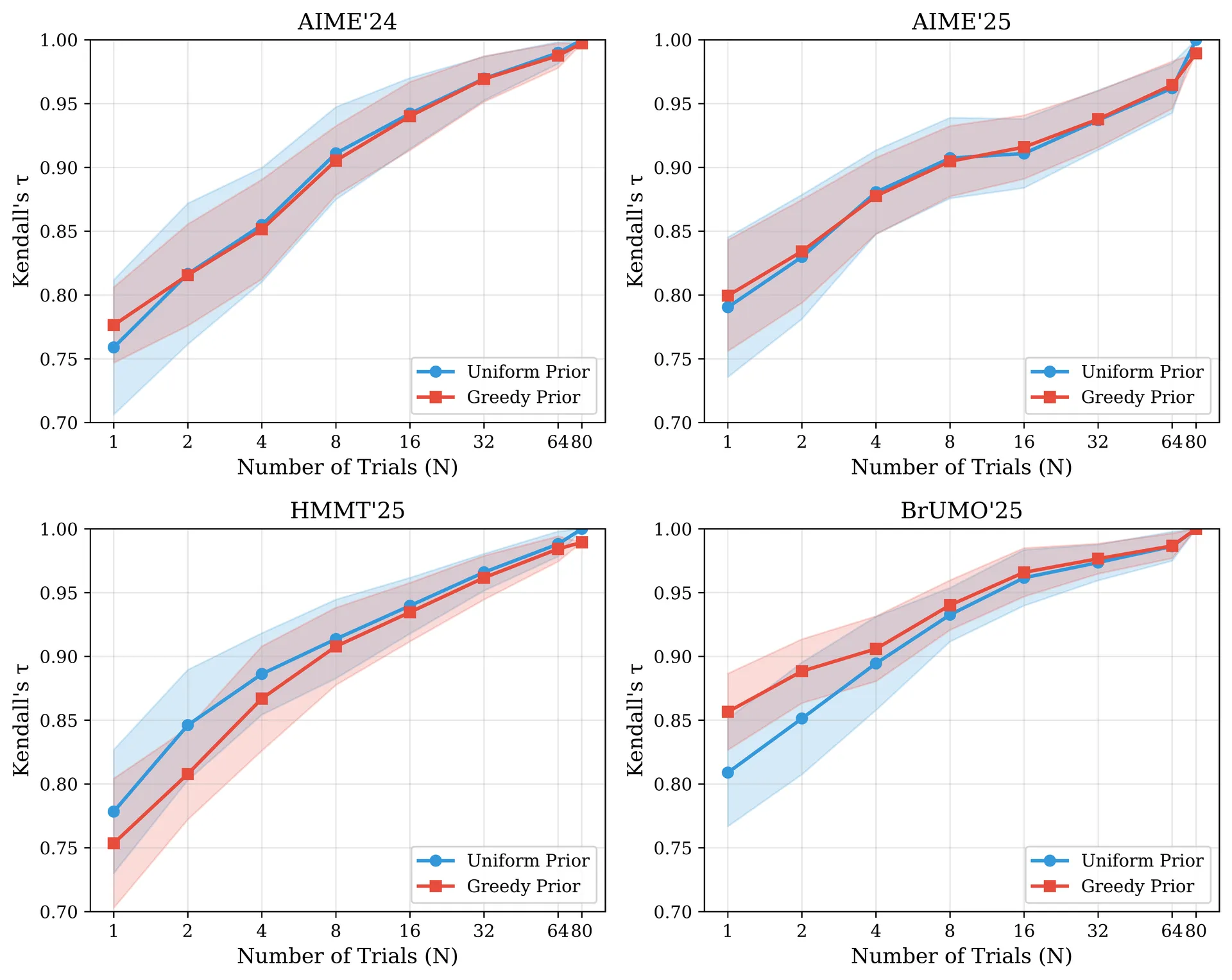
The catch is the mean. Cutting variance is only good if you were aiming at the right target. On three benchmarks the greedy prior nudges the mean up; on HMMT'25, the hardest one, it pushes the ranking away from the accuracy order. The sign of the shift tracks a single diagnostic: how well greedy decoding and stochastic sampling already agree.
| Benchmark | Difficulty | (greedy − uniform) | Std. reduction | |
|---|---|---|---|---|
| AIME'24 | 0.620 | 0.739 | +0.020 | 42% |
| AIME'25 | 0.533 | 0.660 | +0.008 | 17% |
| HMMT'25 | 0.333 | 0.635 | −0.022 | 16% |
| BrUMO'25 | 0.588 | 0.768 | +0.049 | 52% |
is the greedy–sampling rank alignment: Kendall's between the ranking induced by greedy decoding and by stochastic sampling at . Higher alignment goes with a more positive . The prior helps most on BrUMO'25 (aligned, ) and hurts on HMMT'25 (least aligned, ).
# One greedy decode per question, shared across models: shape (M, D)
R0 = np.load("greedy.npy")               # shape (30, 1)

ranking_uniform = rank.bayes(R)          # Bayes_U@N
ranking_greedy  = rank.bayes(R, R0=R0)   # Bayes_R0@N, greedy empirical prior

# Conservative, uncertainty-aware ranking via a posterior lower bound
ranking_lcb = rank.bayes(R, R0=R0, quantile=0.05)
The mechanism is intuitive once you see the scatter of greedy vs. sampled ranks below. Greedy decoding under-explores on hard instances, where stochastic sampling can still stumble onto a correct chain. When the two policies rank models the same way, the prior is free stabilization; when they diverge, it quietly biases the leaderboard toward greedy behavior. That is why the prior is not free information; it changes the target unless you have checked the alignment on a small pilot.
![]()
Beyond binary: categorical ranking has the same trap
The estimator is not limited to right/wrong. Map each completion to one of ordered categories, using signals like boxed-vs-unboxed answers, confidence (bits per token), token efficiency, or an external verifier, and attach a utility weight vector . Bayesian estimation then runs on a Dirichlet–multinomial model instead of Beta–binomial, and rank.bayes(R_cat, w=w) ranks by the weighted posterior mean.
These auxiliary signals reproduce the self-consistency trap in a sharper form. Across categorical schemes at on the combined benchmark, the signal-rich schemes are the most self-consistent (Verifier-only reaches ) yet the least faithful to the accuracy gold standard (). The trade-off is a clean negative correlation: the more a scheme leans on auxiliary signals, the more stable and the more biased it becomes.
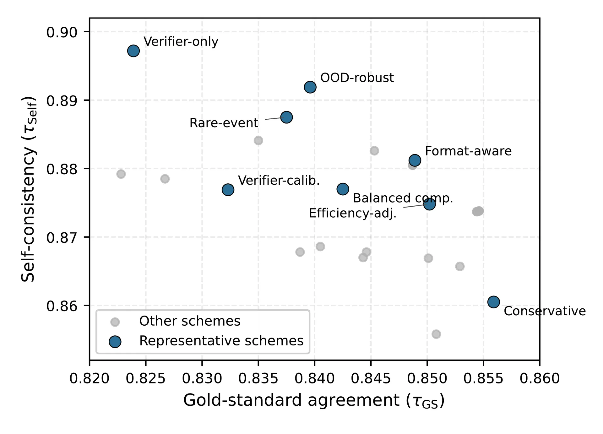
The practical rule that falls out is a reporting discipline: state the category mapping and the utility weights, and never read higher self-consistency as higher accuracy fidelity. All eight representative schemes also correlate more strongly with the greedy-prior reference than the uniform one, the same mechanism as the empirical prior: verifier and format signals partly encode greedy-decoding behavior.
What to actually report
The paper is not a case for one exotic leaderboard. It is a case for a small amount of discipline once evaluation becomes a repeated-sampling problem:
- Name the target. Accuracy agreement, self-consistency, and task-utility rankings are different objects. Decide which one you want before declaring a winner.
- Report stability, not just a point ranking. At low budget, a leaderboard needs , an uncertainty estimate, and convergence as grows.
- Use as the default. It is transparent, order-equivalent to accuracy, and uncertainty-aware. Reach for a greedy prior only after checking greedy–sampling alignment on a pilot sample, and audit any auxiliary signal the same way.
Abstract
Test-time scaling evaluates reasoning LLMs by sampling multiple outputs per prompt, but ranking models in this regime remains underexplored. We formalize dense benchmark ranking under test-time scaling and introduce Scorio, a library that implements statistical ranking methods such as paired-comparison models, item response theory (IRT) models, voting rules, and graph- and spectral-based methods. Across reasoning models on four Olympiad-style math benchmarks (AIME'24, AIME'25, HMMT'25, and BrUMO'25; up to trials), most full-trial rankings agree closely with the Bayesian gold standard (mean Kendall's –), and – methods recover exactly the same ordering. In the single-trial regime, the best methods reach . Using greedy decoding as an empirical prior () reduces variance at by –, but can bias rankings when greedy and stochastic sampling disagree. These results identify reliable ranking methods for both high- and low-budget test-time scaling. We release Scorio as an open-source library at https://github.com/mohsenhariri/scorio.
This is the ranking half of the Bayes@N story, and I am still working on it, extending the analysis past binary correctness to partial credit and rubric-based scoring. If you want to compare notes or you are running your own repeated-trial evaluations, my email is in the footer.