Ranking Reasoning LLMs under Test-Time Scaling

Introduction

figure*[t]

Figures/main_bump_chart_rankings_show_case.pdf Agreement between each method's full-trial ranking and the gold standard. Kendall's ${\tau }_b$ is computed between each method's ranking (at $N=80$ trials) and 80 on an easier benchmark (BrUMO'25, left) and the hardest benchmark (HMMT'25, right). On BrUMO'25, multiple methods achieve near-perfect or perfect agreement: N and HodgeRank reach ${\tau }_b=1.0$, while Rasch MML achieves $0.997$. On HMMT'25, Bradley - Terry and HodgeRank maintain perfect agreement (${\tau }_b=1.0$), but N drops to $0.989$ and Pass@$2$ falls to $0.937$. This divergence is consistent with the lower greedy - sampling alignment observed on harder benchmarks (section 3.4).

figure*

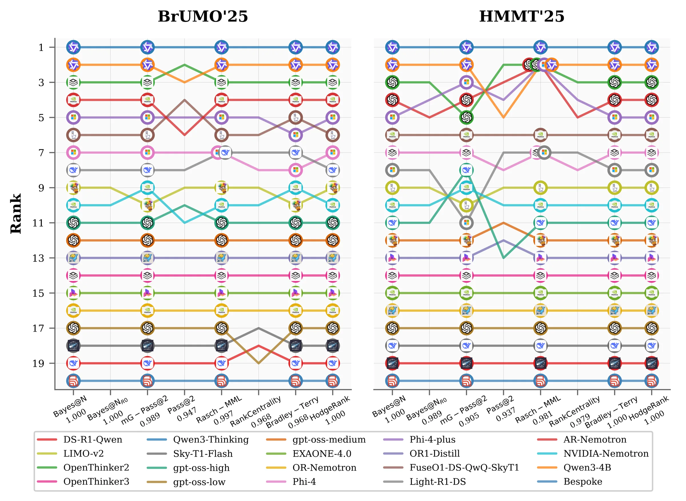
Large language models (LLMs) are increasingly used as general-purpose reasoning systems for tasks such as programming and mathematical problem solving [1, 2]. Reliable evaluation is therefore essential. In many settings, what matters is not only an absolute score but also a ranking that supports model selection, deployment, and scientific comparison. This need is amplified by test-time scaling, which allocates additional inference compute by sampling multiple outputs per prompt and aggregating them, turning evaluation into a repeated-sampling problem [2, 3, 4].

Statistical ranking methods underpin two common LLM workflows. First, preference-based learning and alignment pipelines rely on human or model preferences over alternative responses, where the primitive observations are paired comparisons and downstream optimization depends on how those preferences are modeled and aggregated [5, 6]. Second, model comparisons are often communicated through leaderboards. Crowdsourced paired-comparison platforms such as Chatbot Arena collect head-to-head judgments and fit rating or paired-comparison models to produce public rankings [7], while benchmark-style evaluations rank models by task performance metrics such as Pass@$k$ [1]. Recent work has revisited the statistical foundations of LLM ranking in both preference-based settings [8] and benchmark settings, including IRT-style benchmarking [9]. Different ranking methods can produce noticeably different model orderings, and their agreement can vary with benchmark difficulty (?).

A key practical distinction between these regimes is the representation of the data used for ranking. Preference-based evaluation typically yields a sparse and evolving comparison graph because only a subset of model pairs are compared and the model pool changes over time [7]. In contrast, benchmark evaluations produce dense outcomes for every model - question pair. For a fixed set of $L$ models and $M$ questions, we observe an outcome for every pair. Under test-time scaling, each model - question pair is evaluated with $N$ independent trials, producing a response tensor $\mathbf{R}\in \{0,1{\}}^{L\times M\times N}$. This dense repeated-trial setting raises new methodological questions: Which ranking rule should be used when $N$ is small? How quickly do different ranking methods stabilize as $N$ grows? How do priors and uncertainty estimates affect ranking robustness?

In this work, we study performance-based ranking under test-time scaling. We formalize the dense benchmark setting through the response tensor $\mathbf{R}$, evaluate ranking methods by their low-budget stability and convergence as the test-time budget increases, and implement the studied methods in Scorio.

We summarize our contributions as follows:

• We formalize dense benchmark ranking under test-time scaling via $\mathbf{R}\in \{0,1{\}}^{L\times M\times N}$ and connect common ranking families through pointwise, pairwise, and setwise transformations of $\mathbf{R}$.
• We propose an evaluation protocol based on low-budget stability (agreement between rankings computed from subsampled trials and reference rankings) and convergence with increasing numbers of trials.
• We compare a broad suite of ranking methods across $20$ reasoning models and four Olympiad-style math benchmarks (up to $N=80$ trials), characterizing where method families agree and where they diverge.
• We analyze Bayesian and uncertainty-aware ranking choices, including priors and conservative (quantile-based) scoring, and quantify their bias - variance trade-offs in low-trial regimes.
• We release Scorio, a library implementing the ranking methods and Bayesian options.

Ranking Problem and Test-time Scaling

In classical statistical settings, there is no canonical theoretical ground truth or empirical gold standard against which competing ranking rules can be judged. Choosing among methods therefore usually requires additional modeling assumptions. Test-time scaling offers a useful alternative: because each model - question pair can be sampled repeatedly, it lets us evaluate ranking methods by how stable they are in low-budget settings and how quickly they converge as more trials are observed.

Statistical ranking methods are widely used in domains such as sports competitions (e.g., paired-comparison models and rating systems for head-to-head games) [10, 11, 12] and voting or collective decision-making [13, 14, 15]. In such settings, there are $L$ entities to be ranked (e.g., players, items, or models) over $M$ tasks (e.g., matches, questions, or instances). Test-time scaling adds a third dimension: $N$, the number of i.i.d. samples generated for a fixed question $m\in \{1,\dots ,M\}$. Repeated sampling lets us study two complementary properties. First, low-budget stability asks whether a ranking computed from a small number of trials agrees with a high-budget reference ranking. In our experiments, the low-budget case is $N=1$: we subsample one trial per question, compute the ranking, repeat this over the available single-trial draws, and compare each ranking either with an empirical gold standard or with the same method's full-trial ranking. Second, convergence asks how quickly rankings computed from $n$ trials approach the full-trial ordering as $n$ increases from $1$ to $N$.

Gold Standard Rankings

Evaluation metrics widely used in test-time scaling, such as Pass@$k$ and Bayes@$N$, can be analyzed through statistical properties such as bias. For instance, [1] derive an unbiased estimator for Pass@$k$. As the number of trials $N$ grows, empirical estimates of these metrics concentrate around their population values, making metric-based rankings increasingly stable. In particular, for binary outcomes, N is order-equivalent to mean accuracy avg@$N$ [16], which motivates our use of the full-trial N ranking as an empirical accuracy-based gold standard.

This reasoning does not extend automatically to all ranking methods. Even as the number of questions $M$ or trials $N$ increases, different ranking methods need not converge to a unique limiting ordering, such as the one induced by average accuracy (Appendix 11.1). Unlike evaluation metrics, ranking algorithms can emphasize different aspects of performance across tasks, players, or items. In section 3, we show that rankings induced by probabilistic models (e.g., Bradley - Terry) can differ from those induced by expected-performance metrics (e.g., mean accuracy or Bayesian estimates).

Given the absence of a universal gold standard for ranking methods, we use two target rankings for comparison. First, we define an empirical gold standard based on average performance over all trials with a large sample size (e.g., $N=80$). This target captures aggregate performance across tasks and trials while allowing ties. This choice is justified for several reasons: (a) the ranking induced by average performance is order-equivalent to the ranking induced by Bayesian estimation with a uniform prior (N); (b) when $N$ is large, average performance is among the most stable ranking rules relative to the alternatives (section 3.1); and (c) it is easy to interpret, widely used in practice, and yields absolute performance values.

The second target ranking is the ordering produced by a method itself (method@$80$) when all available trials are aggregated. This target lets us assess a method's self-consistency and convergence as more data become available.

Representation

We consider $L$ models evaluated on a benchmark of $M$ questions under test-time scaling, generating $N$ i.i.d. trials per model - question pair. Let $\mathcal{L}=\{1,\dots ,L\}$ index models and $\mathcal{Q}=\{1,\dots ,M\}$ questions; for each question we observe $N$ independent trials indexed by $n\in \{1,\dots ,N\}$. For each $(l,m,n)\in \mathcal{L}\times \mathcal{Q}\times \{1,\dots ,N\}$ we observe a binary outcome

where $R_{lmn}=1$ if model $l$ solves question $m$ on trial $n$. We collect these outcomes in a response tensor $\mathbf{R}\in \{0,1{\}}^{L\times M\times N}$. When $N=1$, this reduces to the standard single-run benchmark setting. Unlike crowdsourced paired-comparison datasets (e.g., Chatbot Arena [7]), where the primitive observations are model - model outcomes on a possibly sparse comparison graph, our benchmark setting produces outcomes for every model - question pair. We discuss the Arena sparse-comparison counterpart in section 15. We therefore take $\mathbf{R}$ as the primitive object; all ranking methods we study use $\mathbf{R}$ as input, but they differ in the representations on which they operate after transforming or aggregating it.

Pointwise (model - question) representation.

Define the per-question solve rate

and the overall mean accuracy ${\hat{p}}_l:=\frac{1}{M}{\sum }_{m=1}^M{\hat{p}}_{lm}$. Pointwise and IRT-style methods operate on the matrix $\hat{\mathbf{P}}=[{\hat{p}}_{lm}]\in [0,1{]}^{L\times M}$ (or on its row means), optionally reweighting questions (e.g., inverse-difficulty weighting [17]). Classical IRT models infer latent abilities from this representation [18, 19], and have recently been applied to LLM benchmarking [9]. When $N>1$, the trial axis corresponds to repeated Bernoulli observations; likelihood-based models (including IRT) can equivalently work with the sufficient statistic $k_{lm}:={\sum }_n{R}_{lmn}$, yielding a binomial-response formulation [20, 21]. Related repeated-measures and longitudinal IRT extensions are also well studied [22, 23]. Evaluation-metric rankings (e.g., Pass@$k$ and Bayes@$N$) additionally use the per-question trial multiset $\{R_{lm1},\dots ,R_{lmN}\}$ (equivalently the count ${\sum }_n{R}_{lmn}$) to compute per-question metrics before aggregating across $m$ [1].

Pairwise (win/tie) representation.

Many classical ranking methods reduce $\mathbf{R}$ to pairwise outcomes. For a pair of models $(i,j)\in {\mathcal{L}}^2$ we define win and tie counts

so that, in our fully observed setting, $W_{ij}+W_{ji}+T_{ij}=MN$ for all $i\ne j$. Equivalently, we can form an undirected comparison graph $G=(V,E)$ with vertex set $V=\mathcal{L}$ and edge set $E=\{\{i,j\}:W_{ij}+W_{ji}+T_{ij}>0\}$, and store $(W_{ij},W_{ji},T_{ij})$ on each edge. In our benchmark setting $E$ is the complete graph (every pair is compared $MN$ times), whereas in interactive evaluation settings $E$ is typically sparse and one assumes $G$ is connected. The matrices $\mathbf{W}=[W_{ij}]$ and $\mathbf{T}=[T_{ij}]$ define a weighted comparison graph over models. Probabilistic paired-comparison models (e.g., Bradley - Terry and tie extensions [10, 24, 25]) and voting rules (e.g., Borda and Copeland [13, 26]) use these aggregated counts; graph- and spectral-based methods (e.g., PageRank, Rank Centrality, HodgeRank, SerialRank, AlphaRank, and Nash-based ranking [27, 28, 29, 30, 31, 32]) further transform $(\mathbf{W},\mathbf{T})$ into Markov chains or skew-symmetric edge flows, typically via edge weights based on empirical win rates such as ${\hat{P}}_{i\succ j}=(W_{ij}+\frac{1}{2}{T}_{ij})/(W_{ij}+W_{ji}+T_{ij})$. Sequential rating systems (e.g., Elo and TrueSkill [11, 33]) instead process the underlying stream of pairwise "matches" induced by each question - trial $(m,n)$.

Listwise or setwise representation.

For each question - trial $(m,n)$ we define the winning set $U_{mn}:=\{l\in \mathcal{L}:R_{lmn}=1\}$ and the losing set $\mathcal{L}\setminus U_{mn}$, which induces a two-level partial order: all winners tie above all losers. Setwise or listwise models (e.g., Plackett - Luce [34, 35] and Davidson - Luce [36]) operate directly on the collection of events $\{(U_{mn},\mathcal{L}\setminus U_{mn}){\}}_{m,n}$, discarding degenerate events with $U_{mn}=\varnothing$ or $U_{mn}=\mathcal{L}$. In our binary two-level setting, Plackett - Luce likelihoods collapse to functions of pairwise win counts (cf. the MM formulation for generalized Bradley - Terry and Plackett - Luce likelihoods [37]), whereas Davidson - Luce explicitly models within-set ties.

Bayesian Approaches in Ranking

Many ranking methods can be viewed as probabilistic models with latent parameters $\theta$ (e.g., model strength and, optionally, question difficulty). Given observations $\mathbf{R}$ (or derived representations such as pairwise counts; section 2.2), inference reduces to estimating $\theta$ from a likelihood $p(\mathbf{R}\mid \theta )$. We consider maximum likelihood estimation (MLE), maximum a posteriori (MAP), and expected a posteriori (EAP), and discuss how uncertainty can be propagated to rankings [38]. Although MLE is not Bayesian, we include it as a standard baseline for likelihood-based ranking models.

Maximum likelihood estimation (MLE).

The maximum likelihood estimate is

which yields a point estimate without requiring a prior. MLE is attractive for its simplicity, but in paired-comparison and IRT-like models it can be unstable under (near-)separation or weak identification, which motivates priors in MAP and EAP.

Maximum a posteriori (MAP).

MAP incorporates prior information $p(\theta )$ and estimates the posterior mode:

Equivalently, MAP is a penalized MLE in which $-\log p(\theta )$ acts as a regularizer; priors can improve stability in paired-comparison and IRT-style models [39, 40]. We can also construct empirical priors from auxiliary evaluation runs. For example, a prior outcome tensor ${\mathbf{R}}_0$ (e.g., one greedy decode per question) can be used to regularize stochastic trials (EmpiricalPrior in Scorio) [16].

Expected a posteriori (EAP).

EAP uses the posterior mean as the point estimate:

which is Bayes-optimal under squared-error loss [38]. Compared with MAP, EAP accounts for posterior mass beyond the mode and typically requires approximation or sampling. EAP is common in latent-trait settings such as IRT and adaptive testing [41].

Interval estimates and conservative ranking.

Bayesian methods naturally yield credible intervals (posterior quantiles) for each ${\theta }_l$, while frequentist analyses can produce approximate confidence intervals for ${\hat{\theta }}_{\mathrm{MLE}}$ via bootstrap resampling of questions or trials. Interval estimates are especially useful because ranking is sensitive to near ties: rather than ranking by point estimates alone, one can rank conservatively using a lower credible or confidence bound (LCB), or report pairwise superiority probabilities $\mathrm{Pr}({\theta }_i>{\theta }_j\mid \mathbf{R})$. Metric-level Bayesian estimators such as Bayes@$N$ provide both a posterior mean and uncertainty, enabling rankings by posterior mean or by a chosen posterior quantile. Bayes@$N$ also supports incorporating prior outcomes ${\mathbf{R}}_0$ (e.g., one greedy decode per question) as pseudo-counts in the posterior, which is complementary to using ${\mathbf{R}}_0$ to define empirical priors for MAP in parametric ranking models. Our implementation in Scorio supports both credible-interval ranking via Bayes@$N$ and empirical priors via EmpiricalPrior for MAP estimation.

Experiments

We evaluate $72$ ranking methods (Appendix 18.2) on four Olympiad-style math benchmarks: AIME'24, AIME'25, HMMT'25, and BrUMO'25, each with $M=30$ questions. We use $L=20$ reasoning LLMs (full list in table 2). For each model - question pair, we collect $N=80$ independent trials via top-$p$ sampling, yielding a response tensor $\mathbf{R}\in \{0,1{\}}^{20\times 30\times 80}$. We also collect a single greedy-decoding output per question (${\mathbf{R}}_0$) to serve as an empirical prior. Detailed generation, sampling, and reproducibility settings appear in section 17; the library API is documented in section 18.

Gold Standard Ranking

Following section 2.1, we define the gold-standard ranking as 80, the Bayesian posterior-mean estimator with a uniform prior computed from all $N=80$ trials. This choice is order-equivalent to avg@$80$ (mean correctness over all $M$ questions and all $N=80$ trials, with ties allowed) and yields an interpretable accuracy-based target. Empirically, when each of our $72$ ranking methods is computed using all $80$ trials, the resulting orderings agree closely with 80 (?): across benchmarks, the average Kendall's ${\tau }_b$ between 80 and the other methods is $0.93$-$0.95$ (median $0.95$-$0.99$), and $19$-$34$ methods recover exactly the same ordering (${\tau }_b=1$). The largest deviations come from a small set of voting rules (e.g., minimax and Nanson variants) and difficulty-weighted baselines, with minimum ${\tau }_b$ values of $0.68$-$0.79$ depending on the benchmark. Although N is order-equivalent to avg@$N$, we prefer the Bayesian formulation because it supports priors (e.g., N) and uncertainty estimates.

Tables/main_gold_standard_agreement.tex

Ranking-Method Stability

To compare ranking methods in the low-budget regime, we set $N=1$ by subsampling one of the $80$ trials per question and recomputing the rankings. For each method, we report Kendall's ${\tau }_b$ averaged over the $80$ single-trial draws (mean $\pm$ std). Since the Pass@$k$ family requires at least two trials to differ from mean accuracy, the $N=1$ comparisons below cover the remaining $69$ methods.

Gold-standard agreement.

We first rank methods by agreement with the empirical gold standard (80). Across AIME'24, AIME'25, and BrUMO'25, N performs best, achieving ${\tau }_b=0.779\pm 0.034$, $0.798\pm 0.045$, and $0.858\pm 0.028$, respectively (?). On HMMT'25, the hardest benchmark (see section 10), the greedy prior no longer helps, and the best score is shared by a $21$-method equivalence class (N and several graph- and voting-based methods), with ${\tau }_b=0.790\pm 0.053$. When all benchmarks are pooled (Combined), the same $21$-method class attains ${\tau }_b=0.865\pm 0.049$, while N drops to ${\tau }_b=0.786\pm 0.031$ (?).

Self-consistency and convergence.

Next, we evaluate each method against its own full-trial ranking (method@$80$), which summarizes convergence from $N=1$ to $N=80$. Rasch MML with LCB scoring is the most self-consistent on AIME'24, AIME'25, and HMMT'25, with ${\tau }_b=0.804\pm 0.051$, $0.834\pm 0.054$, and $0.810\pm 0.056$ (?); BrUMO'25 again favors N ($0.858\pm 0.028$). On the Combined benchmark, the most self-consistent method is Nanson's rule with tie averaging ($0.892\pm 0.050$), followed by Rasch MML (LCB) ($0.883\pm 0.037$), whereas several minimax variants are among the least self-consistent (down to $0.765\pm 0.045$; ?). High self-consistency does not imply strong agreement with the gold standard: Nanson (avg ties) ranks first in self-consistency on Combined but has substantially lower gold-standard agreement ($0.807\pm 0.036$; ?).

Tables/main_n1_winners.tex

Bootstrapped Model-Pool Robustness

The preceding $N=1$ results use the full set of $20$ models. To test whether those conclusions depend on the evaluation pool, we repeat the low-budget analysis on bootstrapped model pools of size $5$, $10$, and $15$. For each bootstrap subset, we recompute the full-trial rankings, use the subset-specific avg@$80$ ordering as the gold-standard target, and compare each method's $80$ single-trial rankings against two references: (i) the subset-specific avg@$80$ ordering and (ii) its own subset-specific full-trial ranking (method@$80$). We aggregate $1000$ bootstrap subsets for each benchmark - size setting.

Easy and medium benchmarks preserve the original winner.

On AIME'24, AIME'25, and BrUMO'25, N remains the best representative method under both targets at all three model-pool sizes (?). The mean score changes only slightly with pool size: on AIME'24, gold-standard agreement moves from $0.769$ to $0.780$ and self-consistency from $0.773$ to $0.785$ as the pool size increases from $5$ to $15$ models; on AIME'25, the corresponding ranges are $0.797$-$0.802$ and $0.803$-$0.809$; on BrUMO'25, N stays near $0.854$-$0.858$ for both targets. On BrUMO'25, this advantage also becomes more decisive as the pool grows: the fraction of subsets where N is the top-scoring method rises from about $0.69$ at $k=5$ to $0.98$-$0.99$ at $k=15$.

Harder benchmarks remain tie-rich.

The harder settings behave differently. On HMMT'25 and on the Combined benchmark, the top score is not unique: for agreement with avg@$80$, an equivalence class of $29$-$30$ methods shares the best mean, while for method@$80$ the tied class still contains $13$-$14$ methods. We report avg (avg@$N$, order-equivalent to N) as a representative member of these tied classes. The tied optimum is essentially flat across pool size, staying near $0.788$-$0.790$ on HMMT'25 and $0.863$-$0.866$ on Combined. This mirrors the full-model analysis in section 3.2: once the benchmark is difficult or pooled across heterogeneous tasks, many pointwise, voting, and graph-based methods become empirically indistinguishable.

Larger pools mainly reduce between-subset variance.

The primary effect of increasing the model-pool size is to reduce dispersion across subsets rather than to shift the mean systematically (?). For the best method under the avg@$80$ target, the across-subset standard deviation falls from $0.209$ to $0.057$ on AIME'24, from $0.144$ to $0.038$ on AIME'25, from $0.114$ to $0.033$ on HMMT'25, from $0.136$ to $0.032$ on BrUMO'25, and from $0.084$ to $0.023$ on Combined when moving from $5$ to $15$ models. Thus, the qualitative recommendation is stable under moderate changes to the model pool: larger pools mainly make the same conclusion more certain.

Tables/main_model_pool_bootstrap_winners.tex

Effect of Empirical Priors

Empirical priors use auxiliary evaluation signals to stabilize low-budget rankings. In our setting, the signal is a single greedy decode, ${\mathbf{R}}_0$. We incorporate ${\mathbf{R}}_0$ into Bayes@$N$, yielding N, and compare it with the uniform-prior variant N. We evaluate both variants by their agreement with the gold-standard ranking 80. For each $N$, we compute Kendall's ${\tau }_b$ between the induced model ranking and 80 and report the mean and standard deviation over $50$ resampled datasets.

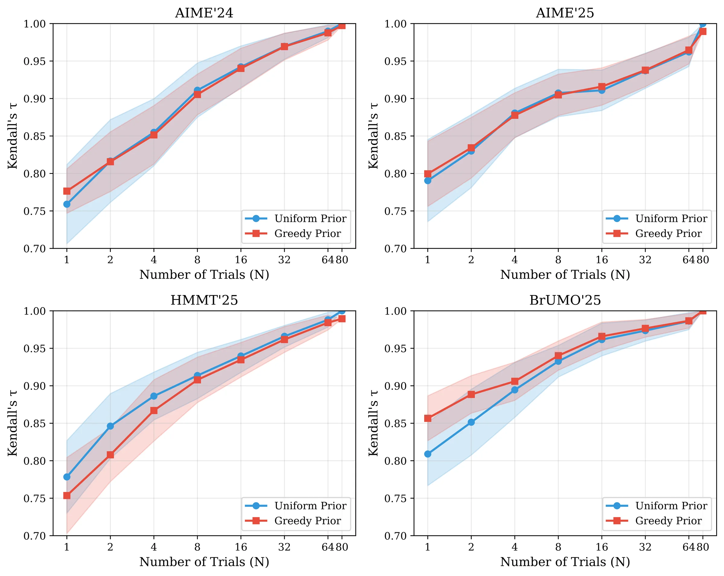
Empirical priors reduce variance at low $N$.

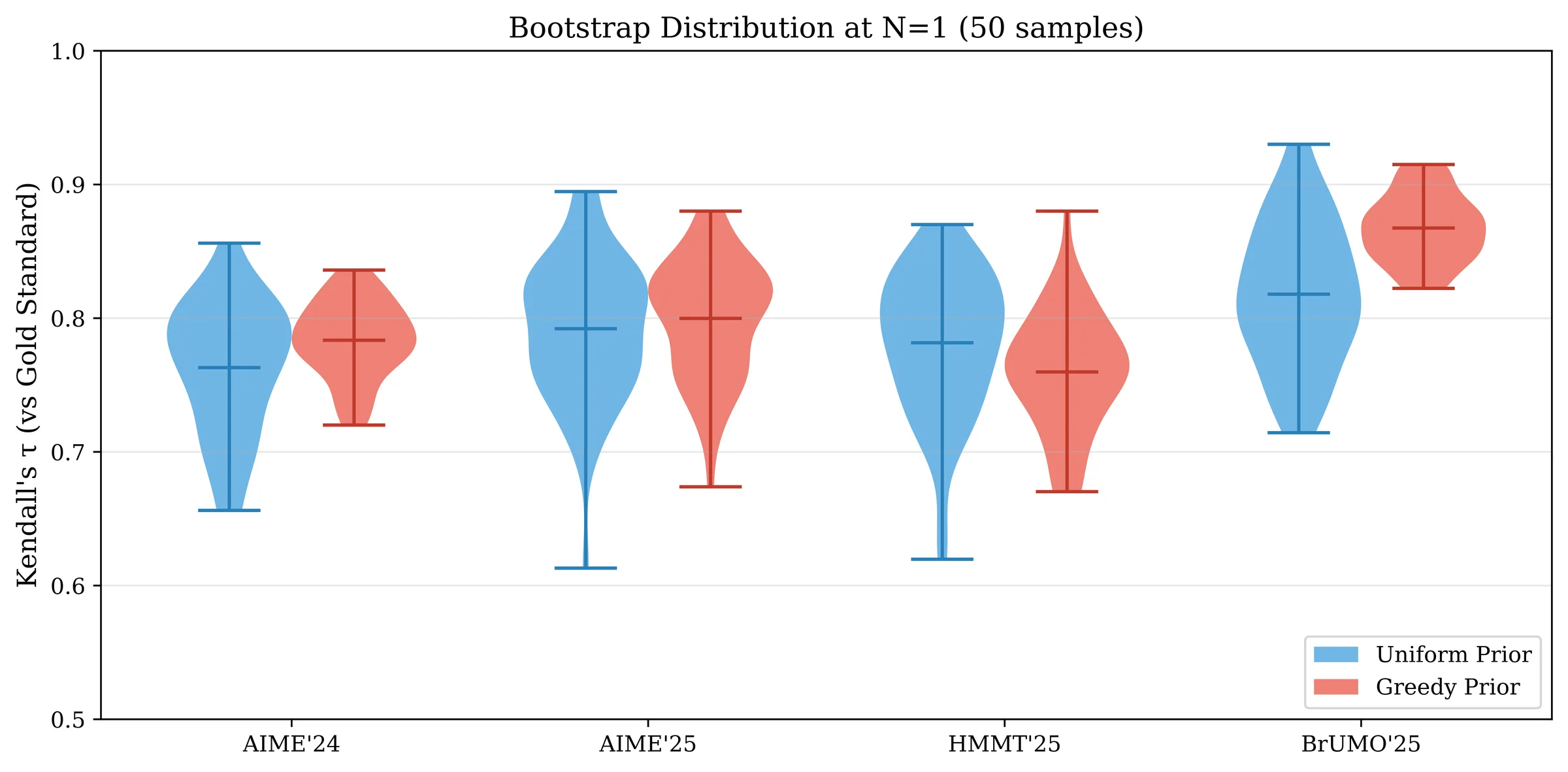
Across all benchmarks, N yields more stable low-$N$ rankings than N. At $N=1$, the standard deviation of ${\tau }_b$ decreases by $16$-$52\%$ depending on the benchmark (table 1, figure 5). This advantage shrinks quickly as $N$ increases (figure 1), consistent with the prior contributing only $O(1)$ pseudo-counts per question.

The mean effect depends on greedy - sampling alignment.

Variance reduction does not guarantee improved agreement with 80. The greedy prior increases mean ${\tau }_b$ on AIME'24, AIME'25, and BrUMO'25, but decreases it on HMMT'25 (table 1). At $N=1$, when all benchmarks are pooled, this negative shift is substantially larger (?), indicating that an empirical prior can introduce systematic bias when greedy and sampling behave differently across datasets.

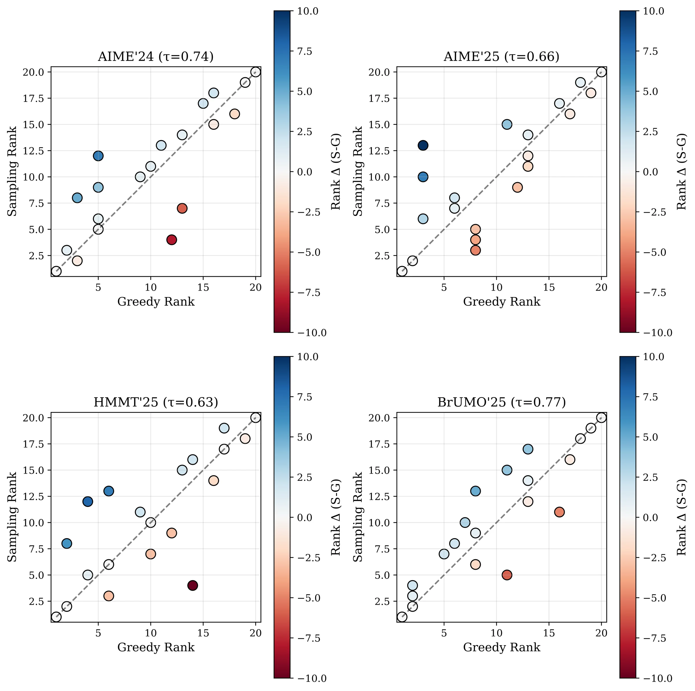
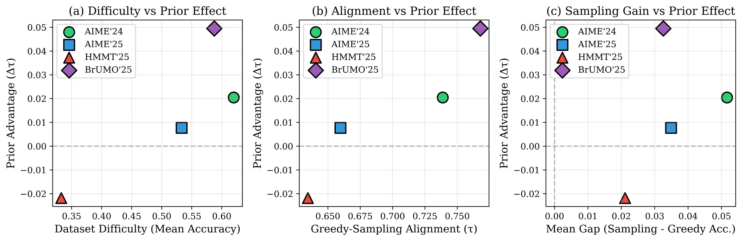
We summarize this diagnostic via greedy - sampling alignment ${\tau }_{\text{G-S}}$, defined as Kendall's ${\tau }_b$ between the model rankings induced by greedy decoding and by stochastic sampling at $N=80$. In our results, higher ${\tau }_{\text{G-S}}$ coincides with a more positive $\Delta \tau$ (section 13, figure 4), suggesting that the empirical prior is most likely to help when greedy is a faithful proxy for the sampling-induced ordering. While this evidence is limited to four benchmarks, the trend is consistent with N acting as shrinkage toward the greedy ordering.

Implications.

N behaves as a shrinkage estimator toward the greedy ordering: it is helpful when greedy decoding is a faithful proxy for the sampling-induced ranking, and harmful when the two disagree. Because ${\mathbf{R}}_0$ is generated under a different decoding policy, incorporating it effectively biases the estimate toward greedy behavior. This can be desirable for variance reduction, but it changes the implied evaluation target. A plausible source of disagreement is that greedy decoding may under-explore on hard instances, while stochastic sampling can recover alternative successful reasoning paths. In practice, empirical priors are most attractive when $N$ is very small and greedy - sampling alignment has been checked on a small pilot sample; otherwise, N provides a safer default.

Bias - variance trade-off.

Figure 5 visualizes the trade-off induced by empirical priors: in our benchmarks, the greedy prior reduces variability (narrower distributions) but can introduce bias (shifted means), with the net effect governed by greedy - sampling alignment.

Categorical Ranking

We extend the Bayesian framework to categorical outcomes: each completion is mapped to one of $C+1$ ordered categories based on signals such as answer format (boxed vs. unboxed), model confidence (completion bits per token), token efficiency, and external verifier judgments. Each scheme defines a categorical mapping and a utility weight vector $\mathbf{w}=(w_0,\dots ,w_C)$; Bayesian estimation then proceeds with a Dirichlet - multinomial model rather than a Beta - binomial model (details and scheme definitions are given in section 14).

We select eight non-redundant representative schemes. Using the $N=1$ subsampling protocol on the Combined benchmark (the first $L=11$ models of table 2, $M=120$ questions pooled across all four datasets), we measure Kendall's ${\tau }_b$ against three references (?).

Tables/main_categorical_combined.tex

Self-consistency vs. gold-standard trade-off.

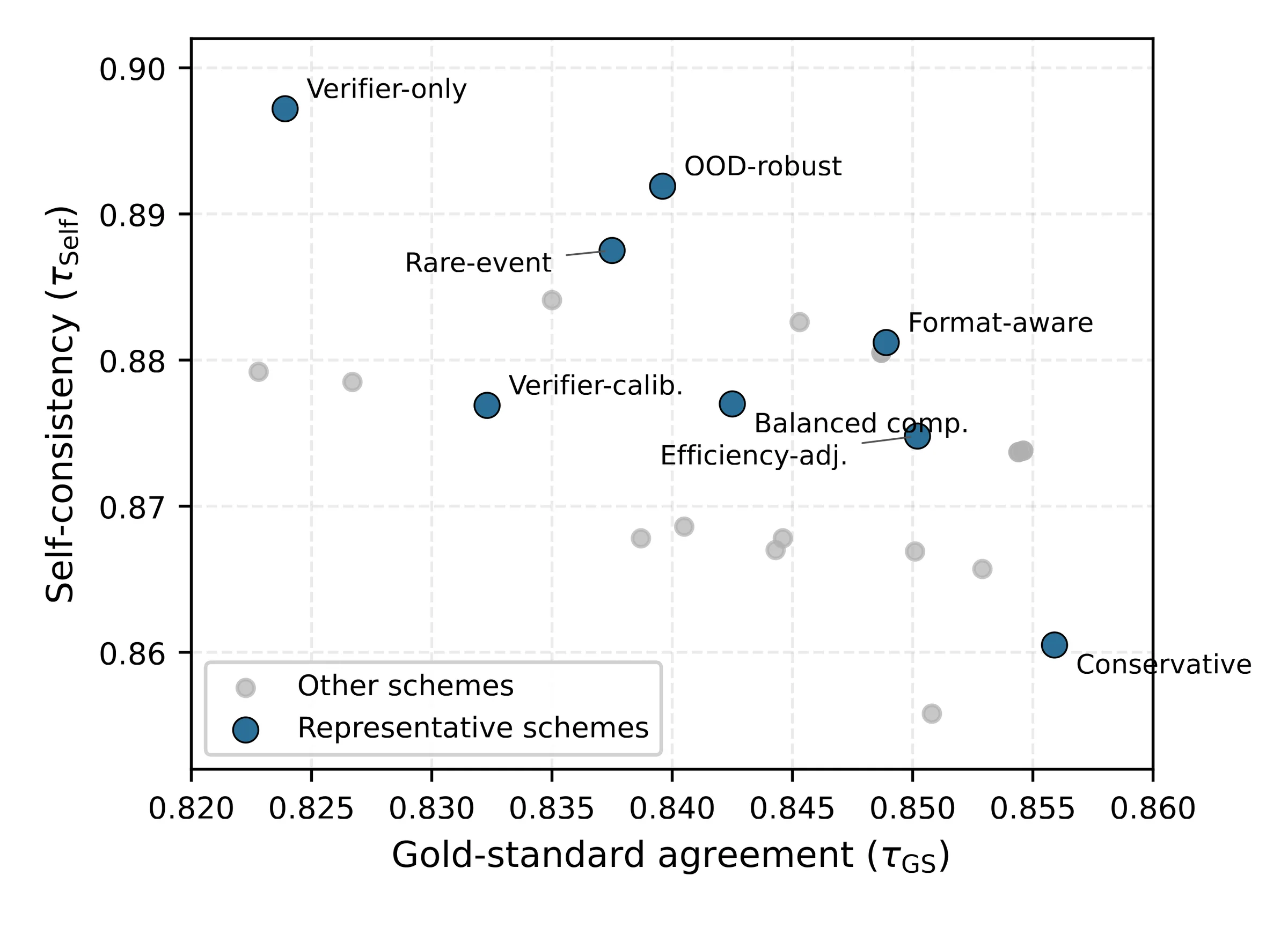
Signal-rich schemes achieve the highest self-consistency: Verifier-only (${\tau }_{\text{Self}}=0.897$) and OOD-robust ($0.892$) rank first and second (figure 3). Yet these schemes have the lowest agreement with the gold standard (${\tau }_{\text{GS}}=0.824$ and $0.840$, respectively), extending the finding from section 3.2 that high self-consistency does not imply closeness to the gold standard. The negative correlation between ${\tau }_{\text{GS}}$ and ${\tau }_{\text{Self}}$ across schemes (figure 3) suggests that auxiliary signals introduce systematic biases away from the correctness-based ordering while stabilizing single-trial rankings.

Greedy-prior alignment.

All eight schemes correlate more strongly with 80 than with 80; the gap is largest for Verifier-only ($\Delta \tau =+0.046$) and OOD-robust ($+0.031$), consistent with the mechanism in section 3.4: verifier and OOD signals encode information partially aligned with greedy-decoding behavior. Per-dataset results (section 14) show that scheme differentiation widens on harder benchmarks (HMMT'25, BrUMO'25), where Verifier-only drops to ${\tau }_{\text{GS}}=0.753$ and $0.734$, while correctness-driven schemes remain stable (${\tau }_{\text{GS}}\ge 0.80$).

Related Work

Test-time scaling samples multiple solutions per prompt and aggregates them [2, 3, 4]; because stochastic reasoning varies across runs [42], we study how this variability affects rankings as budget changes. Preference evaluation and alignment learn from paired comparisons [5, 6] and underpin leaderboards such as Chatbot Arena [7, 8]. Benchmark leaderboards often rank models by task metrics such as Pass@$k$ [1], but item-level difficulty and discrimination affect reliability [43]; recent work adds Bayesian uncertainty and IRT-style modeling [16, 9]. We extend this literature to dense repeated-trial benchmarks and compare ranking methods by stability and convergence; section 16 gives background.

Conclusion & Future Directions

Test-time scaling turns LLM benchmarking into a repeated-sampling problem, so model rankings must be estimated from stochastic trials rather than from a single run. We formalize this setting and compare a broad collection of ranking methods within a common framework. When many trials are available, most reasonable ranking families induce nearly identical orderings, making N a simple and interpretable default. The main differences appear in the low-budget regime. There, uncertainty-aware estimators can improve stability, and the greedy prior N acts as a shrinkage estimator: it reduces variance when greedy and stochastic sampling align, but can bias rankings when they diverge.

In practice, N is a strong default, whereas N is best used after checking greedy - sampling alignment on a small pilot sample. Our experiments focus on binary correctness; extending the analysis to partial credit, rubric-based scoring, and other categorical evaluation settings is a natural next step.

Limitations

Our experiments focus on mathematical reasoning benchmarks. We do not evaluate partial credit, or open-ended outputs, where outcome categories are less clear and annotation or verification noise may be larger. More generally, when informative priors are used - especially priors derived from auxiliary signals other than greedy decoding - the prior source and specification should be reported explicitly, since the prior can introduce systematic bias if it is misaligned with the stochastic evaluation regime.

Acknowledgments

This research was supported in part by NSF awards 2117439 and 2320952.

Appendix

sectionappendix appendixAppendixAppendices appendixAppendixAppendices lstlistingListingListings lstlistingListingListings

Notation and Definitions

Throughout the paper, we use the following notation.

Data and Basic Quantities

• $L$: number of models being ranked.
• $M$: number of questions in a benchmark.
• $N$: number of independent stochastic trials per model - question pair under test-time scaling.
• $\mathbf{R}\in \{0,1{\}}^{L\times M\times N}$: response tensor, where $R_{lmn}=1$ if model $l$ solves question $m$ on trial $n$.
• ${\mathbf{R}}_0$: optional prior outcomes used by Bayesian estimators. In this paper, greedy decoding yields a shared prior matrix ${\mathbf{R}}_0\in \{0,1{\}}^{M\times D}$ with $D=1$, but the notation can also accommodate model-specific prior tensors.
• ${\hat{p}}_{lm}:=\frac{1}{N}{\sum }_{n=1}^N{R}_{lmn}$: per-question solve rate for model $l$ on question $m$.
• $k_{lm}:={\sum }_{n=1}^N{R}_{lmn}$: number of successful trials for model $l$ on question $m$.

Metric Shorthand

• Bayes@$N$: Bayesian posterior-mean estimate at $N$ trials under a specified prior.
• N: Bayesian estimate with a uniform Dirichlet prior, denoted ${\mathrm{Bayes}}_{\mathcal{U}}@N$.
• N: Bayesian estimate with a greedy empirical prior, denoted ${\mathrm{Bayes}}_{{\mathbf{R}}_0}@N$.
• Pass@$k$: probability that at least one of $k$ sampled completions is correct.
• avg@$N$: mean accuracy over all $M$ questions and $N$ trials. For binary outcomes, it is order-equivalent to N.

Ranking-Method Families

• Pointwise methods: aggregate per-question performance to produce model scores (e.g., mean accuracy, inverse-difficulty weighting).
• Pairwise methods: transform outcomes into win/tie counts between model pairs and fit paired-comparison models (e.g., Bradley - Terry, Elo, Glicko).
• Listwise, setwise methods: operate on winner and loser sets for each question - trial (e.g., Plackett - Luce, Davidson - Luce).
• Voting rules: treat questions as voters that rank models and then aggregate those preferences (e.g., Borda, Copeland, Schulze, Kemeny - Young).
• Graph/spectral methods: construct comparison graphs and compute centrality- or flow-based scores (e.g., PageRank, Rank Centrality, HodgeRank, $\alpha$-Rank).
• IRT-inspired methods: estimate latent model abilities and item difficulties (e.g., Rasch, 2PL, 3PL, dynamic IRT).

Evaluation Criteria

• Kendall's ${\tau }_b$: rank-correlation coefficient that accounts for ties; it ranges from $-1$ (perfect disagreement) to $+1$ (perfect agreement).
• Gold-standard agreement: agreement between a low-budget ranking and the empirical gold standard, typically 80 in this paper.
• Self-consistency: agreement between a low-budget ranking and the same method's all-trial ranking.
• Convergence: the rate at which a method's ranking approaches its full-trial ordering as the number of trials increases.
• Greedy - sampling alignment (${\tau }_{\text{G-S}}$): Kendall's ${\tau }_b$ between the ranking induced by greedy decoding and the ranking induced by stochastic sampling at high budget.

Inference Terminology

• MLE (maximum likelihood estimation): point estimate that maximizes $p(\mathbf{R}\mid \theta )$.
• MAP (maximum a posteriori): point estimate that maximizes $p(\mathbf{R}\mid \theta )p(\theta )$.
• EAP (expected a posteriori): posterior mean estimate $\mathbb{E}[\theta \mid \mathbf{R}]$.
• MML (marginal maximum likelihood): likelihood-based estimation that integrates over a latent population distribution, commonly used in IRT.
• Credible intervals (CrI): Bayesian posterior intervals used for uncertainty quantification; we use lower credible bounds (LCBs) for conservative ranking.

Accuracy of Models

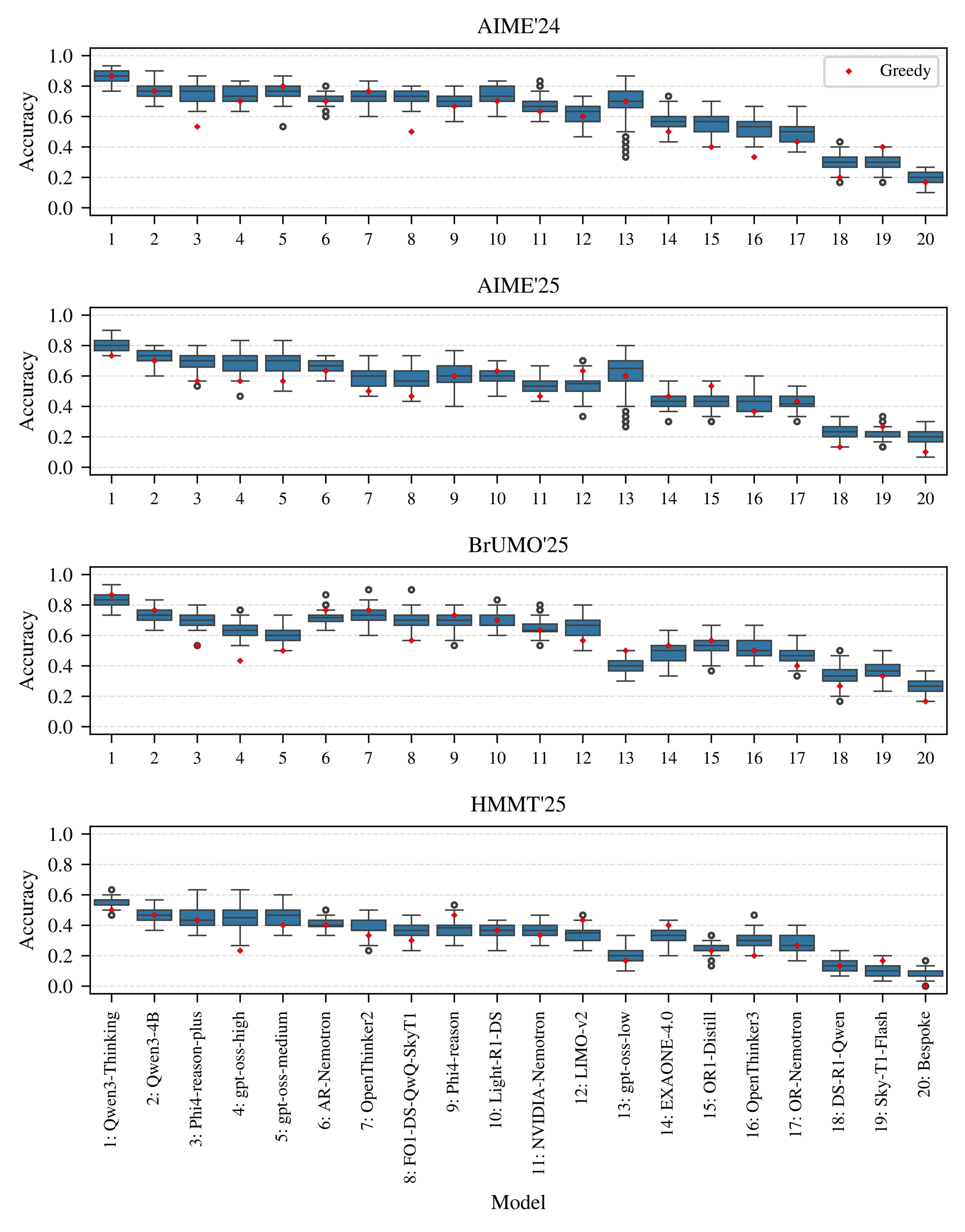
?, ?, ?, ? report detailed accuracy statistics for all $L=20$ models, including greedy accuracy and stochastic-sampling statistics (minimum, mean, maximum, and standard deviation) over $N=80$ trials. HMMT'25 is the most difficult benchmark (mean accuracies $0.080$-$0.554$), whereas AIME'24 and BrUMO'25 are less difficult. ? visualizes these distributions across benchmarks and highlights the heterogeneity in model performance and sampling variance that motivates our ranking-stability analysis.

Tables/appendix_accuracy.tex

figure*[!ht]

Figures/appendix/appendix_acc.pdf Overview of model accuracies across all four benchmarks. Each panel shows each model's mean accuracy under stochastic sampling (over $N=80$ trials), together with greedy accuracy (markers). Error bars denote one standard deviation across trials and illustrate the variability introduced by test-time scaling. Models are color-coded consistently across benchmarks. The figure shows substantial heterogeneity in both absolute performance and sampling variance, with HMMT'25 notably more difficult than the other three benchmarks.

figure*

Gold Standard Agreement

To justify our use of 80 as the gold standard, we compare the full-trial rankings produced by all methods at $N=80$. ? summarizes Kendall's ${\tau }_b$ between 80 and each competing method. These results indicate that 80 is also a high-consensus ordering: by average agreement with all other methods, it ranks first on AIME'25, HMMT'25, and the Combined benchmark and second on AIME'24 and BrUMO'25 within $5\times 10^{-4}$ of the best (?). Dataset-level consensus tables appear in ?, ?, ?, ?, ?. Many methods recover the same ordering exactly (?), and the remaining disagreement is concentrated in a small low-agreement tail (?).

Tables/appendix_gold_standard_consensus.tex Tables/appendix_gold_standard_low_agreement.tex Tables/appendix_aime_kendalltau.tex Tables/appendix_hmmt_kendalltau.tex Tables/appendix_brumo_kendalltau.tex Tables/appendix_combined_kendalltau.tex Tables/appendix_gold_standard_exact_match.tex

Convergence of Ranking Methods

As the number of trials $N$ (or questions $M$) increases, evaluation metrics such as avg@$N$, Bayes@$N$, and Pass@$k$ need not induce the same limiting ordering as ranking methods. The reason is that they target different population quantities.

We illustrate this distinction for two canonical choices used throughout the paper: the average-accuracy ranking and the Bradley - Terry (BT) model.

Large-Budget Limits: Each Method Converges, but Generally to a Different Target

To discuss $M\to \infty$ (or $N\to \infty$) formally, we introduce an i.i.d. sampling model at the level of question - trial pairs. Assume $(X_{mn}{)}_{m\in [M],n\in [N]}$ are i.i.d. draws from some distribution $P$ on $\{0,1{\}}^L$. Let

Here, $p_{\ell }$ depends only on the marginal of model $\ell$, whereas $w_{ij}$ depends on the joint distribution of $(X_i,X_j)$.

Average targets marginal accuracy.

By the law of large numbers,

Likewise, N converges to the same $p_{\ell }$; for binary outcomes it differs from ${\hat{p}}_{\ell }^{\text{avg}}$ only by $O((MN{)}^{-1})$ smoothing.

Bradley - Terry targets a pairwise decisive-win functional.

The empirical win frequencies converge:

Define the BT log-likelihood

Then the BT-ML estimator is an $M$-estimator: maximizing (8) with $W_{ij}$ is equivalent to maximizing the scaled objective $(MN{)}^{-1}\ell (\pi ;W)$. Under mild regularity and connectivity conditions (ensuring strict concavity in $\log \pi$ and uniqueness up to scale), $\hat{\pi }$converges to the unique (up to scale) maximizer of the population objective

The limiting objects $(p_{\ell }{)}_{\ell =1}^L$ and ${\pi }^{\star }$ are generally not linked by any monotone transform: $p_{\ell }$ depends only on marginal correctness, while ${\pi }^{\star }$ depends on the full matrix $(w_{ij}{)}_{i\ne j}$. Therefore, without additional assumptions on $P$ (e.g., that $P$ is generated by a BT choice model at the level of decisive comparisons), there is no reason to expect the induced orderings to coincide as $MN\to \infty$. The following counterexample demonstrates this non-equivalence.

A Counterexample: Average accuracy and Bradley - Terry disagree even at infinite budget

We construct a distribution $P$ (equivalently, a finite pattern that can be repeated) for which the average ranking and the BT-ML ranking disagree. The construction uses $L=3$ models. For notational convenience, we label them $0,1,2$.

Outcome patterns.

Consider the following three outcome vectors in $\{0,1{\}}^3$:

Let $P$ place mass

Equivalently, one may take a deterministic dataset with $M=8$ questions and $N=1$ trial, containing exactly $2$ questions of Type A, $3$ of Type B, and $3$ of Type C; repeating this block preserves both rankings, as established by the derivation.

The marginal success probabilities are

so the average method ranks

For these three types, the decisive-win probabilities $w_{ij}=\mathbb{P}(X_i=1,X_j=0)$ are:

For the finite $M=8,N=1$ realization, the corresponding win counts are $W_{ij}=8w_{ij}$, i.e.,

It remains to show that BT-ML ranks $1>0>2$ for (11), thereby disagreeing with the average ranking.

A convenient characterization of the BT-ML optimum is the standard first-order condition equating observed wins to model-implied expected wins: for each $i$,

(These equations follow by differentiating (8) with respect to $\log {\pi }_i$.)

Because BT strengths are identifiable only up to a global scale factor, fix ${\pi }_2=1$ and write ${\pi }_0=a$, ${\pi }_1=b$. Plugging (11) into (12) yields two independent equations:

Step 1: solve $a$ in terms of $b$.

From (?),

The left-hand side simplifies:

Thus,

Step 2: determine $b$ from a one-dimensional equation.

Substitute (14) into (13). The substitution gives

so the first term in (13) becomes $5\cdot \frac{a}{a+b}=\frac{3b}{b+1}$. Also,

Therefore (13) is equivalent to

Simplifying gives the cubic equation

Let $f(b)=2b^3-5b^2-16b-15$. We have

so there exists a root $b^{\star }\in (4,5)$. Moreover,

whose positive root is $b=\frac{5+\sqrt{121}}{6}=\frac{16}{6}=\frac{8}{3}$. Hence $f$ is strictly increasing for all $b>\frac{8}{3}$, implying the root $b^{\star }\in (4,5)$ is unique. We therefore conclude that the BT-ML solution (under ${\pi }_2=1$) satisfies $b=b^{\star }\in (4,5)$ and $a=\frac{3(b^{\star }{)}^2}{2b^{\star }+5}$.

Step 3: show $b>a>1$, hence BT ranks $1>0>2$.

Using (14),

Thus, $b>a$ holds exactly when $(2b+5)/(3b)>1$, i.e., when $b<5$. Since $b^{\star }\in (4,5)$, we have $b^{\star }>a$.

It remains to show $a>1$. Suppose for contradiction that $a\le 1$. We have already established $b>a$, so $b\ge a$. Then $\frac{a}{a+b}\le \frac{a}{2a}=\frac{1}{2}$ and $\frac{a}{a+1}\le \frac{1}{2}$. Plugging into (13) gives

a contradiction. Hence $a>1={\pi }_2$. Putting these inequalities together yields

so BT ranks

This contradicts the average ranking $0>1>2$, establishing that the two methods can induce different orderings even in the absence of sampling noise.

From a Finite Counterexample to "No Convergence" as $M\to \infty$ or $N\to \infty$.

The counterexample rules out a general theorem forcing average and BT rankings to coincide in the large-budget limit. To connect it directly to $M\to \infty$ or $N\to \infty$, it suffices that both methods are invariant under replication.

Replication invariance (deterministic construction).

Let $R$ be any fixed tensor. For an integer $k\ge 1$, define: (i) question replication $R^{(k,M)}$ by repeating the $M$ questions $k$ times (so $M^{\prime }=kM$ and $N^{\prime }=N$), and (ii) trial replication $R^{(k,N)}$ by repeating the $N$ trials $k$ times (so $M^{\prime }=M$ and $N^{\prime }=kN$). Then:

1. Average scores are unchanged: \[ p^avg_(R^(k,M))=p^avg_(R^(k,N))=p^avg_(R). \]
2. The decisive-win matrix scales linearly: align* W(R^(k,M)) &= kW(R) \\ W(R^(k,N)) &= kW(R). align*
3. The BT-ML maximizer is unchanged, because the log-likelihood scales as \[ (; kW) = k(;W), \] and therefore has the same maximizer.

Therefore, if two methods disagree on $R$, they disagree on $R^{(k,M)}$ for arbitrarily large $M$ and on $R^{(k,N)}$ for arbitrarily large $N$. Applied to the $M=8,N=1$ tensor corresponding to (11), this yields an explicit sequence with $M\to \infty$ (or $N\to \infty$) for which the average and BT rankings remain different at every budget.

Stochastic formulation (i.i.d. construction).

Alternatively, under the i.i.d. model of section 11.2, the same discrepancy appears at the population level. For the distribution $P$ in section 11.2.3, the limiting average ranking is determined by $(p_{\ell })$ and yields $0>1>2$, while the limiting BT ranking is determined by the maximizer of (9) and yields $1>0>2$. Thus, even with independent sampling and $MN\to \infty$, the two rankings can converge to different limits.

Implications and Support for the Gold-Standard Definition

This analysis has a direct implication for benchmarking ranking methods: there is no method-independent guarantee that all reasonable procedures converge to the same ordering as the evaluation budget grows. Different ranking procedures correspond to different statistical targets.

Why this happens.

Average-based ranking targets the marginal success probabilities $p_{\ell }=\mathbb{P}(X_{\ell }=1)$. BT instead targets the latent strengths that best explain the decisive pairwise win rates $w_{ij}=\mathbb{P}(X_i=1,X_j=0)$ through a logistic choice model. These are different summaries of the same joint outcome distribution $P$. The counterexample in section 11.2.3 isolates the mechanism: a model can have higher marginal accuracy while assigning less decisive-win mass against another model, which shifts the BT optimum.

Why a gold standard is needed.

Because ranking methods need not share a common asymptotic ordering, claims about "distance to the truth" require a specified target ordering. Otherwise even statements such as "method $A$ converges faster than method $B$" are ambiguous.

Our choice: N.

We define the gold-standard ordering as N (with $N=80$ in our experiments). This definition is supported by three considerations:

1. Interpretability and decision relevance. N estimates the probability that a model solves a randomly drawn benchmark item under the sampling policy. This is an accuracy-like quantity with a direct operational meaning.
2. Minimal modeling assumptions. N (and avg@$N$) depend only on marginal correctness and do not impose a parametric pairwise-choice model. Methods such as BT are useful when the pairwise-choice model is appropriate, but their induced ordering is not, in general, a refinement of accuracy.
3. Consistency under increasing budget. Under i.i.d. sampling of $(m,n)$ pairs, N converges to $p_{\ell }$ as $MN\to \infty$, making it a natural "infinite-budget" reference for accuracy-based evaluation.

Relationship to self-consistency.

This non-convergence result does not argue against BT or other rankers. It instead clarifies that two evaluations are complementary: agreement with an explicit accuracy-based target, and self-consistency, i.e., how quickly a method stabilizes toward its own full-budget ordering. The former asks whether a method matches the chosen reference; the latter asks how stable the method itself becomes as trials accumulate. The counterexample shows why these questions are not interchangeable.

Minimality of the eight-question construction

The counterexample in Section 11.2.3 uses $M=8$ questions. The same setting ($L=3$, $N=1$, and BT-ML fit from decisive wins) also yields a minimality fact: there is no strict disagreement example with fewer than eight questions.

Proposition (minimal $M$ for strict disagreement; verified by exhaustive enumeration).

Assume $L=3$ and $N=1$. Assume moreover that the average ranking is strict (all three average scores are distinct), and that BT-ML is well-defined and finite (equivalently, the directed win graph with an edge $i\to j$ whenever $W_{ij}>0$ is strongly connected, which ensures a unique BT-ML maximizer up to global scale). If BT-ML disagrees with the average ranking, then $M\ge 8$.

Verification.

With $N=1$, each question produces an outcome pattern in $\{0,1{\}}^3$. Hence, up to permutation of questions, any dataset with $M$ questions is determined by the count vector $c=(c_x{)}_{x\in \{0,1{\}}^3}\in {\mathbb{N}}^8$ with ${\sum }_x{c}_x=M$. For fixed $M$, there are $\left(\genfrac{}{}{0ex}{}{M+7}{7}\right)$ such vectors; thus the total number of datasets with $M\le 7$ is

For each such dataset, we compute the induced average ordering and the BT-ML ordering (obtained by maximizing (8), equivalently solving (12)). Restricting to datasets with (i) strict average ordering and (ii) strong connectivity (so the BT-ML maximizer is unique up to scale), an exhaustive enumeration yields $1506$ instances for $M\le 7$; in all of them the BT-ML ordering agrees with the average ordering. Therefore, no strict-disagreement example exists for $M\le 7$.

Section 11.2.3 exhibits a strict-disagreement dataset at $M=8$, so $M_{\min }=8$.

Ranking-Method Stability at $N=1$N=1

We provide additional details for the $N=1$ stability analyses in section 3.2. Method rankings on the Combined benchmark are reported for (i) gold-standard agreement (method@1 vs. 80) and (ii) self-consistency (method@1 vs. method@80), collapsing method variants with identical mean and standard deviation across the 80 single-trial draws.

As a pair-level diagnostic, we compute gap-conditional stability: pooled over benchmarks, 1 reversals concentrate among near-tied pairs under the 80 gap $g_{ij}=|{\mu }_i-{\mu }_j|$ ($g_{ij}\le 0.02$: reversal $0.350$, tie $0.151$, pairwise correctness $0.566$), while well-separated pairs are ordered almost perfectly ($g_{ij}\ge 0.10$: correctness $0.985$; $g_{ij}\ge 0.20$: correctness $0.999$).

Tables/appendix_n1_gs_combined.tex Tables/appendix_n1_self_combined.tex

Additional Prior Diagnostics

Supplementary diagnostics for the empirical-prior analysis in section 3.4 are shown in figure 4, figure 5.

Categorical Ranking

We report the experimental setup and per-dataset results for the categorical-ranking experiments summarized in section 3.5.

Setup

The binary Bayesian estimator (section 2.3) models each trial outcome as $R_{lmn}\in \{0,1\}$ and places a Beta prior on the per-question solve rate. The categorical extension maps each completion to one of $C+1$ categories, yielding outcomes $R_{lmn}\in \{0,\dots ,C\}$ defined by auxiliary signals extracted during generation. A categorical scheme $s$ specifies:

1. a categorical mapping ${\varphi }_s:\text{completion features}\to \{0,\dots ,C_s\}$, which assigns each completion to a category based on predicates over the base signals (?), and
2. a utility weight vector ${\mathbf{w}}_s=(w_0,\dots ,w_{C_s})\in {\mathbb{R}}^{C_s+1}$, encoding the relative value of each category.

Bayesian estimation replaces the Beta - binomial model with a Dirichlet - multinomial model: for each model - question pair, a symmetric Dirichlet prior is placed on the $C+1$ category probabilities $\mathbf{\theta }=({\theta }_0,\dots ,{\theta }_C)$, and the posterior mean of the weighted utility ${\sum }_{k=0}^C{w}_k{\hat{\theta }}_k$ is computed. Model-level scores are then aggregated across questions, as in the binary case.

Base signals.

For each of the $L=11$ models in the categorical cohort, we extract $9$ features per completion (?). These features span five domains: answer format (has_box), correctness (is_correct), generation cost (token_ratio, repeated_pattern), decoding confidence (prompt_bpt, completion_bpt), and external verification via CompassVerifier (compass_A/B/C). The feature tensors have shape $(N,M,9)$ per model, with $N=80$ trials and $M=30$ questions per benchmark.

CompassVerifier CompassVerifier-3B provides the external verification signals. Its scores on completions generated by the other models define the verifier-based categorical schemes. Verifier inference uses Transformers [44] and Accelerate [45], with FlashAttention kernels [46] and the DFloat11 format [47] for throughput.

Tables/appendix_categorical_signals.tex

Derived predicates and thresholds.

Several predicates are shared across schemes. All thresholds are computed per-model from the available samples:

• Invalid: $\text{repeated\_pattern}=1$ or $\text{compass\_C}\ge 0.5$.
• Confidence: High confidence $:=$$\text{completion\_bpt}\le P_{40}(\text{completion\_bpt})$; wrong - high-confidence $:=$ wrong and $\text{completion\_bpt}\le P_{60}(\text{completion\_bpt}\mid \text{wrong})$.
• Prompt OOD: $\text{prompt\_bpt}\ge P_{90}(\text{prompt\_bpt})$.
• Efficiency bands: Economical/moderate/verbose based on $P_{33}$ and $P_{66}$ of $\text{token\_ratio}$.
• Verifier: CompassVerifier dominant label is $\arg \max (A,B,C)$; verifier-high $:=$$A\ge 0.6$.

Scheme definitions.

The experiments include $25$ categorical schemes spanning correctness-only baselines (A, H, S, Y), confidence-aware (C, I, J, V), format-aware (B, P, T), efficiency-aware (F, G, M), verifier-based (D, K, O, U, Z), OOD-aware (E, N, W), abstention-aware (L, Q), and composite (R) variants. Several schemes are metric-level near-duplicates (e.g., A $\equiv$ S, H $\equiv$ Y, L $\equiv$ Q), so the reported comparison uses $8$ non-redundant representative schemes covering distinct design axes (?).

Tables/appendix_categorical_schemes.tex

Evaluation protocol.

For each scheme, we apply the same $N=1$ subsampling protocol as in section 3.2: one of the $N=80$ trials is subsampled per question, the scheme's categorical ranking is computed, and Kendall's ${\tau }_b$ is measured against three references:

1. Gold-standard (${\tau }_{\text{GS}}$): agreement with the binary 80 ranking, which treats outcomes as correct/wrong with a uniform Dirichlet prior.
2. Self-consistency (${\tau }_{\text{Self}}$): agreement with the scheme's own all-$80$-trial ranking (Scheme@$80$).
3. Greedy-prior (${\tau }_{\text{Greedy}}$): agreement with 80, the binary Bayes ranking incorporating a greedy-decoding empirical prior.

Statistics (mean and standard deviation) are computed over the $80$ single-trial draws. Combined results aggregate the four benchmarks ($M=120$ questions) and are reported in ?; per-dataset results are reported in ?.

Per-Dataset Results

? reports gold-standard agreement and self-consistency for each benchmark separately. The results show three main patterns.

Tables/appendix_categorical_per_dataset.tex

Narrow spread on individual benchmarks.

On each benchmark individually, all eight schemes achieve ${\tau }_{\text{GS}}$ between $0.73$ and $0.83$, with inter-scheme variation much smaller than on the combined benchmark. On AIME'24, the range across the $8$ schemes is only $0.007$ ($0.813$-$0.820$). This narrow spread reflects the limited information available from a single trial with $M=30$ questions and $L=11$ models; the combined benchmark ($M=120$) offers finer discrimination among category structures.

Verifier-only degrades on hard benchmarks.

The Verifier-only scheme exhibits the largest performance drop on the harder benchmarks: ${\tau }_{\text{GS}}$ falls from $0.813$ (AIME'24) to $0.753$ (HMMT'25) and $0.734$ (BrUMO'25), a decline of $0.06$-$0.08$. In contrast, correctness-driven schemes (Conservative, Efficiency-adjusted, Format-aware) remain above $0.80$ on all benchmarks. This pattern suggests that CompassVerifier judgments are less reliable proxies for correctness on more challenging problems.

Self-consistency converges to gold-standard on individual benchmarks.

On AIME'24, the self-consistency column is nearly identical to the gold-standard column for most schemes, indicating that the all-$80$ scheme ranking coincides with the binary 80 ranking when the number of questions is small. On the combined benchmark (?), self-consistency consistently exceeds gold-standard agreement, reflecting convergence of each scheme to its own distinct ordering when given enough questions.

Arena Ranking

Our experiments consider a dense benchmark tensor $\mathbf{R}\in \{0,1{\}}^{L\times M\times N}$: every model is evaluated on every question, and repeated stochastic trials provide multiple binary outcomes for each model - question pair. Arena evaluation, exemplified by preference leaderboards such as Chatbot Arena, uses a different observation model. Its primitive datum is a comparison among a small set of model responses to a prompt, so the data form a sparse, possibly time-varying comparison graph rather than a complete model - question - trial tensor. We analyze how the ranking families studied in this work transfer to this sparse-comparison regime, and where additional assumptions are required.

Observation Model

Let

denote a pairwise Arena log. At comparison $t$, models $a_t,b_t\in \{1,\dots ,L\}$ respond to prompt $x_t$; a human or model judge returns $y_t\in \{a_t\succ b_t,b_t\succ a_t,a_t\sim b_t\}$; and ${\omega }_t\ge 0$ is an optional weight for reliability, deduplication, or target-distribution reweighting. Writing $i{\succ }_{t}j$ for the event that model $i$ is preferred to model $j$ in comparison $t$, let ${\mathcal{T}}_{ij}=\{t:\{a_t,b_t\}=\{i,j\}\}$. We define

with $W_{ii}=T_{ii}=0$ and $C_{ij}=W_{ij}+W_{ji}+T_{ij}$. These counts induce the comparison graph

In the dense benchmark setting, each question - trial pair induces pairwise outcomes for all model pairs, so $G$ is complete and $C_{ij}=MN$ for every $i\ne j$. Arena ranking removes this completeness assumption: only co-observed models contribute to an edge, and missing comparisons should not be interpreted as losses.

Which Ranking Families Transfer

Methods whose sufficient statistics are pairwise comparisons transfer most directly. For example, Bradley - Terry estimation on Arena data uses the same win counts as in the dense reduction. Let

The log-likelihood is

Tie-aware variants such as Davidson or Rao - Kupper additionally use $T_{ij}$. Sequential rating systems (Elo, Glicko, TrueSkill) can be run directly on the timestamped comparison stream, whereas the dense benchmark setting must first expand each question - trial slice into induced pairwise matches.

Graph and spectral methods also transfer after estimating pairwise preference probabilities on observed edges, for example

where $\alpha \ge 0$ is a smoothing constant. These edge weights can be used by PageRank, Rank Centrality, HodgeRank, $\alpha$-Rank, and related graph-based procedures. Hodge-style decompositions are diagnostically useful because they separate a global ranking potential from cyclic residuals, which may reveal non-transitive preferences caused by prompt specialization, heterogeneous judges, or context-dependent model strengths. If an Arena compares more than two responses to the same prompt, the event may instead be represented by winner and loser sets $(U_t,V_t)$ and passed to listwise or setwise Luce-family models.

Pointwise metrics do not transfer without additional labels. Mean accuracy, Pass@$k$, Bayes@$N$, and standard IRT models require absolute model - item outcomes, whereas a preference log records only relative judgments. A response can win a comparison without being correct, or lose to a stronger response despite being acceptable. If the Arena protocol also records absolute signals - for example correctness, rubric scores, verifier labels, or categorical response features - then the problem becomes a masked benchmark rather than a pure preference arena. In that case, pointwise or IRT-style likelihoods can be written over the observed entries only,

where $A$ is the observation mask. The mask is essential: zero-filling unobserved entries would conflate non-participation with failure and bias rankings toward frequently sampled models.

Sparsity also changes the role of regularization. In dense benchmarks, every model pair receives the same number of induced comparisons. In an Arena, low-degree models and disconnected components may be weakly identified or incomparable from data alone. Priors, anchor models, or a small dense benchmark pilot can therefore be more important for Arena ranking than for the controlled dense benchmark setting.

Evaluation Under Comparison Budgets

The stability protocol in section 3 extends to Arena logs by replacing the trial budget $N$ with a comparison budget. For a ranking method $r$, let

Agreement between ${\pi }_r(t)$ and ${\pi }_r(T)$, measured for example by Kendall's ${\tau }_b$, gives the Arena analogue of low-budget stability and convergence. Prefix evaluation preserves time order and measures how quickly a live leaderboard stabilizes; bootstrap evaluation resamples comparisons, prompts, or user sessions to quantify uncertainty. When observations share prompts, users, or judges, resampling at those higher levels is preferable to treating all comparisons as independent.

Arena rankings should be interpreted conditionally on the prompt distribution, judge population, model-selection policy, and decoding policy used to collect the log. Reporting should therefore include both rank estimates and diagnostics: connectivity and degree statistics of $G_{\mathrm{arena}}$, edge-count imbalance, posterior or bootstrap intervals for model strengths, and pairwise superiority probabilities such as $\mathrm{Pr}({\theta }_i>{\theta }_j\mid {\mathcal{D}}_{\mathrm{arena}})$. Randomizing presentation order, maintaining anchor models, and stratifying by prompt domain make the estimand more transparent and reduce artifacts from side bias or adaptive sampling.

Arena ranking is therefore the sparse-comparison counterpart of the dense repeated-trial setting. The ranking estimators need not be redesigned when they operate on pairwise or setwise sufficient statistics; the observation model and uncertainty structure instead change because comparisons are sparse, non-uniform, and evolving. In Scorio, Arena logs correspond to sparse win/tie matrices or setwise events that can be processed by the paired-comparison, graph, or listwise rankers analyzed in this work.

Extended Related Work

Test-time scaling produces repeated stochastic outcomes per item, making LLM benchmarking closer to classical repeated-measurement settings than to single-run leaderboards. We summarize the main ranking families used in this work and their typical applications.

Paired-comparison and rating models.

Paired-comparison models represent comparisons through win/tie counts and infer latent strengths, with Bradley - Terry as a canonical likelihood-based model [10]. Practical systems often use online rating updates such as Elo and its extensions (e.g., Glicko) or fully Bayesian skill ratings such as TrueSkill [11, 12, 33]. For data with ties, common generalizations include Rao - Kupper and Davidson models [24, 25]. These models are widely used for preference aggregation in LLM leaderboards [7, 8], but are also natural in dense benchmarks once per-item outcomes are reduced to pairwise wins.

Listwise, setwise choice models.

When each trial yields an ordering over many items, listwise choice models such as Plackett - Luce provide a likelihood over permutations [34, 35]. Davidson - Luce extends setwise choice to allow ties within selected sets [36]. In our binary benchmark setting, each trial induces a two-level partition (solved vs. unsolved), so these models reduce to structured forms of pairwise likelihoods while still providing a principled view of aggregation.

IRT and difficulty-aware benchmarking.

Item response theory models couple model "ability" with item difficulty (and sometimes discrimination), with the Rasch and Birnbaum formulations as classic examples [18, 19]. IRT has recently been proposed as a way to disentangle model skill from benchmark composition in LLM evaluation [9]. When multiple trials per item are available, repeated-measures extensions and binomial-response formulations are natural [21, 22, 23], and difficulty reweighting has also been explored in NLP evaluation contexts [17].

Graph, spectral, and social-choice methods.

Beyond likelihood-based models, ranking from comparisons has a long tradition in social choice and graph-based aggregation. Voting rules such as Borda and Condorcet-style methods satisfy different axioms and can behave differently under noise and ties [13, 14, 15, 26]. Spectral and Markov-chain approaches derive scores from transition graphs, including PageRank and Rank Centrality [27, 28]; HodgeRank and related spectral methods interpret comparisons as edge flows and decompose them into global and cyclic components [29, 30]. AlphaRank was introduced for multi-agent evaluation with potentially non-transitive interactions [31], and related work studies open-ended evaluation dynamics [32]. We place these families in a common test-time-scaling benchmark setting and compare them under controlled increases in the number of repeated trials.

Experiment Setup and Reproducibility

Models and Datasets

Datasets.

We evaluate on four Olympiad-style math benchmarks: AIME'24 [48], AIME'25 [49], BrUMO'25 [50], and HMMT'25 [51]. For AIME'24 and AIME'25, we combine AIME I and AIME II from the corresponding year, yielding $30$ integer-answer problems per benchmark. For HMMT'25, we use the official February 2025 contest set, which spans algebra, geometry, number theory, and combinatorics. For BrUMO'25, we use the published 2025 problem sets from the tournament archive.

Models.

To reduce prompt-format confounds, we use provider-recommended chat templates (defaulting to DeepSeek/Qwen-style templates when no model-specific template is given) and shared decoding settings across models unless noted otherwise. We evaluate the $20$ models listed in table 2: Sky-T1-32B-Flash Sky-T1-32B-Flash [52] (Sky-T1 Flash release), Qwen Qwen3-30B-A3B-Thinking-2507 [53] (Qwen3 thinking model), DeepSeek DeepSeek-R1-Distill-Qwen-1.5B [54] (1.5B distilled reasoning model), gpt-oss gpt-oss-20b [55] (OpenAI open-weight model, evaluated with low, medium, and high Harmony reasoning effort under the default MXFP4 quantization), LIMO LIMO-v2 [56] (reasoning model), EXAONE EXAONE-4.0-1.2B [57] (hybrid reasoning/non-reasoning model), NVIDIA OpenReasoning-Nemotron-1.5B [58] (NVIDIA reasoning model), OpenThinker OpenThinker2-32B [59] and OpenThinker OpenThinker3-1.5B [59] (models trained from the OpenThoughts data recipes), Microsoft Phi-4-reasoning and Microsoft Phi-4-reasoning-plus [60], OpenR1 OpenR1-Distill-7B [61], FuseO1 FuseO1-DeepSeekR1-QwQ-SkyT1-Flash-32B-Preview [62], Light-R1 Light-R1-14B-DS [63], NVIDIA AceReason-Nemotron-1.1-7B [64], NVIDIA NVIDIA-Nemotron-Nano-9B-v2 [65], Qwen Qwen3-4B-Thinking-2507 [53], and Bespoke-Stratos Bespoke-Stratos-7B [66].

Prompting.

We use provider-recommended prompt templates for each model. For most models, we adopt the standard DeepSeek/Qwen-style prompt, "Please reason step by step, and put your final answer within boxed\\." For gpt-oss gpt-oss-20b, we use the OpenAI Harmony prompt template, which specifies three discrete levels of reasoning effort. For NVIDIA OpenReasoning-Nemotron-1.5B, we use the task-specific prompt, "Solve the following math problem. Make sure to put the answer (and only the answer) inside boxed\\."

Reproducibility

For stochastic runs, we use top-$p$ sampling with temperature $0.6$, $p=0.95$, batch size $1$, and random seeds $1234$ through $1313$, yielding $N=80$ trials per dataset - model pair. All models are served with vLLM (PagedAttention) [67] in bf16 precision, except releases that require MXFP4 quantization (e.g., gpt-oss). We record log-probabilities for both input prompts and generated tokens, with max_tokens set to $32,768$. All experiments run on clusters equipped with $8\times$ NVIDIA H200 GPUs (141GB per GPU).

Computational Cost and Token Statistics

We evaluate 20 models across four benchmarks, with 80 trials per model and 30 questions per benchmark, for a total of 192,000 independent inference runs. The full evaluation requires 7,445 GPU-hours (approximately 310 GPU-days) and generates 2.96B tokens (2,963,318,176 total); table 3 reports the task-level totals. Of these tokens, 37M (1.2%) are prompt tokens and 2.93B (98.8%) are completion tokens, for an average of 15,434 tokens per query. Among the four benchmarks, HMMT'25 is the most computationally expensive at 2,217 GPU-hours, whereas BrUMO'25 is the least expensive at 1,651 GPU-hours. Across model configurations, gpt-oss-20b-low is the most efficient (48.4 GPU-hours for 9,600 queries) and LIMO-v2 the least efficient (894.3 GPU-hours for the same workload), with a corpus-wide average of 139.6 seconds per query.

Rank Correlation Metrics

Kendall's tau

Kendall's tau ($\tau$) [68] measures ordinal agreement between two rankings through pairwise concordance and discordance. For rankings of $n$ items, let $n_c$ and $n_d$ denote the numbers of concordant and discordant pairs, let $n_0=n(n-1)/2$ be the total number of pairs, and let $n_1$ and $n_2$ be the numbers of tied pairs in the two rankings. The two common variants are

Tau-a ignores ties, whereas Tau-b corrects for them. Because ties are common in our setting, we use ${\tau }_b$ throughout.

Scorio, Open-Source Library for LLM Ranking

Scorio is a Python library for ranking LLMs from repeated-trial benchmark evaluations under test-time scaling. It provides a unified interface for mapping the response tensor $\mathbf{R}\in \{0,1{\}}^{L\times M\times N}$ (and, where relevant, optional prior outcomes) to model scores and rankings across evaluation metrics, probabilistic paired-comparison and rating systems, voting rules, listwise choice models, item response theory, and graph- or spectral-based methods. The library is distributed through PyPI as scorio.

All ranking methods in Scorio operate on the response tensor $\mathbf{R}$, where $L$ is the number of models, $M$ the number of questions, and $N$ the number of trials per question. The implementation represents this tensor as a NumPy array of shape (L, M, N). ? gives a minimal example of constructing $\mathbf{R}$ and calling a basic ranking method.

import numpy as np
from scorio import rank

# Binary response tensor: L=3 models, M=4 questions, N=5 trials
R = np.random.randint(0, 2, size=(3, 4, 5))

# Rank by mean accuracy
rankings = rank.avg(R)

# Return both rankings and scores
rankings, scores = rank.avg(R, return_scores=True)

The rank module uses a common interface: each function takes the tensor $\mathbf{R}$ as the first argument, returns a ranking array of shape (L,), and accepts an optional return_scores=True flag to additionally return the underlying scores. Rankings are $1$-indexed, with lower values indicating better models.

Scorio implements ranking methods from several families. ? illustrates evaluation-based methods, including the Pass@$k$ family that quantifies how reliably models solve questions within $k$ sampled trials.

# Pass@k: probability at least 1 of k draws succeeds
rankings, scores = rank.pass_at_k(R, k=3, return_scores=True)

# G-Pass@k with threshold tau
rankings = rank.g_pass_at_k_tau(R, k=5, tau=0.6)

# Bayesian posterior ranking with optional prior outcomes
R0 = np.random.randint(0, 2, size=(3, 4, 2))  # prior data
rankings = rank.bayes(R, R0=R0)

The bayes method generalizes beyond binary correctness to categorical outcomes $R_{lmn}\in \{0,\dots ,C\}$ via a weight vector $\mathbf{w}\in {\mathbb{R}}^{C+1}$ that maps each category to a score. It also accepts an optional prior tensor ${\mathbf{R}}_0$ that incorporates outcomes from a different evaluation setting (e.g., greedy decoding) as a Bayesian prior. ? gives examples of both cases.

# Categorical outcomes: 0=wrong, 1=partial, 2=correct
# L=3 models, M=4 questions, N=5 trials
R_cat = np.random.randint(0, 3, size=(3, 4, 5))

# Weight vector mapping categories to scores
w = np.array([0.0, 0.5, 1.0])

rankings, scores = rank.bayes(R_cat, w=w,
                              return_scores=True)

# Using greedy decoding results as Bayesian prior
# R0 shape (M, D): shared prior across all models
R0_greedy = np.random.randint(0, 3, size=(4, 2))
rankings = rank.bayes(R_cat, w=w, R0=R0_greedy)

# Conservative ranking via posterior quantile
rankings = rank.bayes(R_cat, w=w, R0=R0_greedy,
                      quantile=0.05)

For probabilistic paired-comparison models, Scorio implements the Bradley - Terry model and its extensions, as well as Elo and TrueSkill rating systems (?). These methods construct pairwise comparisons from $\mathbf{R}$ and estimate latent strength parameters.

# Bradley-Terry maximum likelihood
rankings, scores = rank.bradley_terry(R, return_scores=True)

# Bradley-Terry with MAP regularization
rankings = rank.bradley_terry_map(R, prior=1.0)

# Elo rating system
rankings, scores = rank.elo(R, K=32.0, return_scores=True)

# TrueSkill Bayesian rating
rankings = rank.trueskill(R)

Graph-based and spectral methods rank models by analyzing the structure of a pairwise comparison graph derived from $\mathbf{R}$, as shown in ?.

# PageRank on the pairwise win-probability graph
rankings, scores = rank.pagerank(R, damping=0.85,
                                 return_scores=True)

# Spectral ranking (principal eigenvector)
rankings = rank.spectral(R)

# Rank centrality via Markov chain stationary distribution
rankings = rank.rank_centrality(R)

A family-wise list of ranking methods is given in section 18.1, and the exact method configurations used in our experiments are reported in section 18.2.

Ranking Methods

Pointwise Methods

Mean accuracy.

The simplest pointwise score is the mean accuracy

which corresponds to avg in Scorio.

Inverse-difficulty weighting.

To emphasize hard questions, inverse_difficulty weights each question by the inverse of its global solve rate $p_m:=\frac{1}{LN}{\sum }_{l,n}{R}_{lmn}$:

with weights normalized to ${\sum }_m{w}_m=1$.

$R\0,1\^L M N$, $>0$
Scores $sR^L$
State Compute $p_lm 1N_n=1^N R_lmn$
State Mean: $s_l 1M_m=1^M p_lm$
State Inv-diff: compute $p_m 1LN_l,nR_lmn$
State Set $w_m 1/clip(p_m,,1-)$ and normalize to $_m w_m=1$
State $s_l _m w_mp_lm$

Evaluation-metric Methods

These methods rank models by evaluation metrics computed from per-question trial outcomes. The simplest baseline is mean accuracy (avg; section 18.1.1); we next define Pass@$k$-family metrics and Bayes@$N$. For a fixed model $l$, define the per-question success counts ${\nu }_{lm}:={\sum }_{n=1}^N{R}_{lmn}$. Each metric defines a per-question score $f({\nu }_{lm};N)$ (or $f({\nu }_{lm};N,k,\tau )$) and then averages across questions.

Pass@$k$ (pass_at_k).

Pass@$k$ [1] is the probability that at least one of $k$ samples is correct. For each question $m$,

and the model-level score is $s_l^{Pass@k}:=\frac{1}{M}{\sum }_{m=1}^{M}Pass@k_{lm}$.

Pass-hat@k / G-Pass@k (pass_hat_k).

This metric (also called G-Pass@k in parts of the recent LLM evaluation literature [69]) is the probability that all $k$ selected samples are correct:

with $s_l^{\widehat{Pass@k}}:=\frac{1}{M}{\sum }_{m=1}^M{\widehat{Pass@k}}_{lm}$.

G-Pass@k${}_{\tau }$ (g_pass_at_k_tau).

G-Pass@k${}_{\tau }$ [42] generalizes these metrics by requiring at least $j_0:=\lceil \tau k\rceil$ successes among the $k$ selected samples. Let $X_{lm}\sim \mathrm{Hypergeom}(N,{\nu }_{lm},k)$ be the number of successes in a draw of size $k$ without replacement; then

and $s_l^{\mathrm{G}\text{-}Pass@k_{\tau }}:=\frac{1}{M}{\sum }_{m=1}^M\mathrm{G}\text{-}Pass@k_{\tau ,lm}$. Scorio defines the endpoint $\tau =0$ to recover Pass@$k$ (and for any $\tau \in (0,1/k]$ the threshold $j_0=\lceil \tau k\rceil$ equals $1$, so the expression matches Pass@$k$), while $\tau =1$ recovers Pass-hat@k.

mG-Pass@k (mg_pass_at_k).

mG-Pass@k [42] aggregates G-Pass@k${}_{\tau }$ over $\tau \in [0.5,1]$. In Scorio, we use the equivalent expectation form

where $(x{)}_{+}:=\max (x,0)$ and $X_{lm}\sim \mathrm{Hypergeom}(N,{\nu }_{lm},k)$. The model-level score is $s_l^{\mathrm{mG}\text{-}Pass@k}:=\frac{1}{M}{\sum }_{m=1}^M\mathrm{mG}\text{-}Pass@k_{lm}$.

Bayes@$N$ (bayes).

Bayes@$N$ [16] applies to multi-category outcomes $R_{lmn}\in \{0,\dots ,C\}$ with a weight vector $w\in {\mathbb{R}}^{C+1}$. For a fixed model $l$ and question $m$, let $n_{mk}:={\sum }_{n=1}^{N}1\{R_{lmn}=k\}$ be category counts. Optionally, a prior outcome matrix $R_0\in \{0,\dots ,C{\}}^{M\times D}$ contributes pseudo-counts $n_{mk}^0:=1+{\sum }_{d=1}^{D}1\{(R_0{)}_{md}=k\}$ (a Dirichlet$(1,\dots ,1)$ prior), giving ${\nu }_{mk}:=n_{mk}+n_{mk}^0$ and $T:=1+C+D+N$. Bayes@$N$ returns a posterior mean ${\mu }_l$ and uncertainty ${\sigma }_l$ of the weighted score:

Scorio ranks by ${\mu }_l$ (default) or by a conservative normal-quantile score ${\mu }_l+{\Phi }^{-1}(q){\sigma }_l$ for a chosen $q\in [0,1]$.

Bayesian Methods

Thompson sampling ranking (thompson).

Thompson sampling [70, 71] ranks by Monte Carlo samples from a conjugate Beta - Binomial posterior over each model's aggregate success probability. We model $p_l\sim \mathrm{Beta}(\alpha ,\beta )$ and treat all $MN$ trials as i.i.d. Bernoulli outcomes [38]. Let $S_l:={\sum }_{m=1}^M{\sum }_{n=1}^N{R}_{lmn}$ be the total number of successes for model $l$; then

For $t=1,\dots ,T$ we draw $p_l^{(t)}\sim p_l\mid \mathbf{R}$ independently for each model, compute the induced rank $r_l^{(t)}\in \{1,\dots ,L\}$ (smaller is better), and score by the negative average rank

Bayesian Bradley - Terry via MCMC (bayesian_mcmc).

To obtain a full Bayesian posterior over paired-comparison strengths, we combine the Bradley - Terry likelihood [10] with a Gaussian prior and approximate the posterior with Metropolis - Hastings sampling [72, 73]. We first form decisive win counts

ignoring ties (both correct or both incorrect). Parameterizing ${\pi }_i=\exp ({\theta }_i)$, the BT likelihood is

with an independent prior ${\theta }_i\sim \mathcal{N}(0,{\sigma }^2)$ [39]. We sample from $p(\theta \mid \mathbf{W})$ and rank models by the posterior mean score $s_i^{\mathrm{MCMC}}:=\mathbb{E}[{\theta }_i\mid \mathbf{W}]$.

Voting-based Methods

Voting rules aggregate per-question preferences into a global ranking. To adapt them to our test-time-scaling setting, we treat each question $m$ as a "voter" that ranks models by their per-question solve frequency across trials:

When $N=1$, each question induces only a two-level ranking (correct vs. incorrect), so Borda/Copeland reduce to (ties of) accuracy-based ordering; when $N>1$ these rules exploit the additional resolution from $k_{lm}$.

Borda count.

For each question $m$, let $r_{lm}\in \{1,\dots ,L\}$ be the (tie-averaged) rank of model $l$ when sorting $k_{\cdot m}$ in descending order (smaller rank is better). The Borda score is

which assigns $(L-1)$ points for a unique first place and $0$ for a unique last place, with ties receiving the average of the tied positions [13, 26].

Copeland.

For each pair $(i,j)$, define the number of questions that prefer $i$ to $j$ as $W_{ij}^{(q)}:={\sum }_m\mathbb{I}[k_{im}>k_{jm}]$. Copeland declares $i$ to beat $j$ if $W_{ij}^{(q)}>W_{ji}^{(q)}$ and scores each model by net pairwise dominance:

References

- Evaluating Large Language Models Trained on Code. misc. 2021. https://arxiv.org/abs/2107.03374
- Self-Consistency Improves Chain of Thought Reasoning in Language Models. International Conference on Learning Representations. 2023. https://openreview.net/forum?id=1PL1NIMMrw
- Scaling LLM Test-Time Compute Optimally can be More Effective than Scaling Model Parameters. misc. 2024. https://arxiv.org/abs/2408.03314
- Revisiting the Test-Time Scaling of o1-like Models: Do they Truly Possess Test-Time Scaling Capabilities?. Proceedings of the 63rd Annual Meeting of the Association for Computational Linguistics (Volume 1: Long Papers). 2025. https://aclanthology.org/2025.acl-long.232/
- Deep Reinforcement Learning from Human Preferences. Advances in Neural Information Processing Systems. 2017. https://papers.nips.cc/paper/7017-deep-reinforcement-learning-from-human-preferences
- Direct Preference Optimization: Your Language Model is Secretly a Reward Model. Advances in Neural Information Processing Systems. 2023. https://papers.nips.cc/paper_files/paper/2023/hash/a85b405ed65c6477a4fe8302b5e06ce7-Abstract-Conference.html
- Chatbot Arena: An Open Platform for Evaluating LLMs by Human Preference. Proceedings of the 41st International Conference on Machine Learning. 2024. https://proceedings.mlr.press/v235/chiang24b.html
- A Statistical Framework for Ranking LLM-based Chatbots. International Conference on Learning Representations. 2025. https://openreview.net/forum?id=rAoEub6Nw2
- Lost in Benchmarks? Rethinking Large Language Model Benchmarking with Item Response Theory. misc. 2025. https://arxiv.org/abs/2505.15055
- Rank Analysis of Incomplete Block Designs: The Method of Paired Comparisons. Biometrika. 1952. https://doi.org/10.1093/biomet/39.3-4.324
- The Rating of Chessplayers, Past and Present. Arco Publishing. 1978. https://archive.org/details/ratingofchesspla0000eloa
- Parameter Estimation in Large Dynamic Paired Comparison Experiments. Journal of the Royal Statistical Society: Series C (Applied Statistics). 1999. https://doi.org/10.1111/1467-9876.00159
- M\'emoire sur les \'elections au scrutin. misc. 1781. https://webusers.imj-prg.fr/ alexandre.guilbaud/LX2U1/Borda_Memoire_sur_les_elections_au_scrutin_MARS_1781_extrait.pdf
- Essai sur l'application de l'analyse `a la probabilit\'e des d\'ecisions rendues `a la pluralit\'e des voix. Imprimerie Royale. 1785. https://archive.org/details/bub_gb_RzAVAAAAQAAJ
- Social Choice and Individual Values. John Wiley & Sons. 1951.
- Don't Pass@k: A Bayesian Framework for Large Language Model Evaluation. Proceedings of the 14th International Conference on Learning Representations (ICLR 2026). 2026. https://openreview.net/forum?id=PTXi3Ef4sT
- Taking the Correction Difficulty into Account in Grammatical Error Correction Evaluation. Proceedings of the 28th International Conference on Computational Linguistics. 2020. https://aclanthology.org/2020.coling-main.188/
- Probabilistic Models for Some Intelligence and Attainment Tests. Danish Institute for Educational Research. 1960. https://archive.org/details/probabilisticmod0000rasc
- Some Latent Trait Models and Their Use in Inferring an Examinee's Ability. Statistical Theories of Mental Test Scores. 1968. https://faculty.ucmerced.edu/jvevea/classes/290_21/readings/week%209/Birnbaum.pdf
- Generalized Linear Models. Springer. 1989. https://doi.org/10.1007/978-1-4899-3242-6
- Explanatory Item Response Models. Springer. 2004. https://doi.org/10.1007/978-1-4757-3990-9
- A Dynamic Generalization of the Rasch Model. Psychometrika. 1993. https://doi.org/10.1007/BF02294648
- On Longitudinal Item Response Theory Models: A Didactic. Journal of Educational and Behavioral Statistics. 2020. https://doi.org/10.3102/1076998619882026
- Ties in Paired-Comparison Experiments: A Generalization of the Bradley - Terry Model. Journal of the American Statistical Association. 1967. https://doi.org/10.1080/01621459.1967.10482901
- On Extending the Bradley - Terry Model to Accommodate Ties in Paired Comparison Experiments. Journal of the American Statistical Association. 1970. https://doi.org/10.1080/01621459.1970.10481082
- Handbook of Computational Social Choice. Cambridge University Press. 2016. https://doi.org/10.1017/CBO9781107446984
- The PageRank Citation Ranking: Bringing Order to the Web. techreport. 1999. https://ilpubs.stanford.edu/422/1/1999-66.pdf
- Rank Centrality: Ranking from Pairwise Comparisons. Operations Research. 2017. https://doi.org/10.1287/opre.2016.1534
- Statistical Ranking and Combinatorial Hodge Theory. Mathematical Programming. 2011. https://doi.org/10.1007/s10107-010-0419-x
- Spectral Ranking using Seriation. Journal of Machine Learning Research. 2016. https://jmlr.org/papers/v17/16-035.html
- -Rank: Multi-Agent Evaluation by Evolution. Scientific Reports. 2019. https://doi.org/10.1038/s41598-019-45619-9
- Open-ended Learning in Symmetric Zero-sum Games. Proceedings of the 36th International Conference on Machine Learning. 2019. https://proceedings.mlr.press/v97/balduzzi19a.html
- TrueSkill: A Bayesian Skill Rating System. Advances in Neural Information Processing Systems. 2006. https://papers.neurips.cc/paper/3079-trueskilltm-a-bayesian-skill-rating-system.pdf
- The Analysis of Permutations. Applied Statistics. 1975. https://doi.org/10.2307/2346567
- Individual Choice Behavior: A Theoretical Analysis. John Wiley & Sons. 1959. https://archive.org/details/individualchoice0000luce
- Davidson - Luce Model for Multi-item Choice with Ties. misc. 2019. https://arxiv.org/abs/1909.07123
- MM Algorithms for Generalized Bradley - Terry Models. The Annals of Statistics. 2004. https://doi.org/10.1214/aos/1079120141
- Bayesian Data Analysis. CRC Press. 2013. https://doi.org/10.1201/b16018
- Efficient Bayesian Inference for Generalized Bradley - Terry Models. Journal of Computational and Graphical Statistics. 2012. https://doi.org/10.1080/10618600.2012.638220
- Bayes Modal Estimation in Item Response Models. Psychometrika. 1986. https://doi.org/10.1007/BF02293979
- A Comparison of Maximum Likelihood Estimation and Expected a Posteriori Estimation in CAT Using the Partial Credit Model. Educational and Psychological Measurement. 1998. https://doi.org/10.1177/0013164498058004002
- Are Your LLMs Capable of Stable Reasoning?. Findings of the Association for Computational Linguistics: ACL 2025. 2025. https://aclanthology.org/2025.findings-acl.905/
- Evaluation Examples are not Equally Informative: How should that change NLP Leaderboards?. Proceedings of the 59th Annual Meeting of the Association for Computational Linguistics and the 11th International Joint Conference on Natural Language Processing (Volume 1: Long Papers). 2021. https://aclanthology.org/2021.acl-long.346/
- Huggingface's transformers: State-of-the-art natural language processing. arXiv preprint arXiv:1910.03771. 2019. https://arxiv.org/abs/1910.03771
- Accelerate: Training and inference at scale made simple, efficient and adaptable.. misc. 2022. https://github.com/huggingface/accelerate
- Flashattention-2: Faster attention with better parallelism and work partitioning. arXiv preprint arXiv:2307.08691. 2023. https://arxiv.org/abs/2307.08691
- 70% Size, 100% Accuracy: Lossless LLM Compression for Efficient GPU Inference via Dynamic-Length Float (DFloat11). Advances in Neural Information Processing Systems. 2025. https://arxiv.org/abs/2504.11651
- American Invitational Mathematics Examination (AIME). misc. 2024. https://maa.org/maa-invitational-competitions/
- American Invitational Mathematics Examination (AIME). misc. 2025. https://maa.org/maa-invitational-competitions/
- Brown University Math Olympiad (BrUMO). misc. 2025. https://www.brumo.org/tournament-info
- HMMT February 2025 Archive (Problems and Solutions). misc. 2025. https://www.hmmt.org/www/archive/282
- Think Less, Achieve More: Cut Reasoning Costs by 50% Without Sacrificing Accuracy. misc. 2025. https://novasky-ai.github.io/posts/reduce-overthinking/
- Qwen3 Technical Report. misc. 2025. https://arxiv.org/abs/2505.09388
- DeepSeek-R1 incentivizes reasoning in LLMs through reinforcement learning. Nature. 2025. https://doi.org/10.1038/s41586-025-09422-z
- gpt-oss-120b & gpt-oss-20b Model Card. misc. 2025. https://arxiv.org/abs/2508.10925
- LIMO: Less is More for Reasoning. Second Conference on Language Modeling. 2025. https://openreview.net/forum?id=T2TZ0RY4Zk
- EXAONE 4.0: Unified Large Language Models Integrating Non-reasoning and Reasoning Modes. misc. 2025. https://arxiv.org/abs/2507.11407
- OpenReasoning-Nemotron-1.5B. misc. 2025. https://huggingface.co/nvidia/OpenReasoning-Nemotron-1.5B
- OpenThoughts: Data Recipes for Reasoning Models. misc. 2025. https://arxiv.org/abs/2506.04178
- Phi-4-reasoning Technical Report. misc. 2025. https://arxiv.org/abs/2504.21318
- Open-R1: A Fully Open Reproduction of DeepSeek-R1. misc. 2025. https://github.com/huggingface/open-r1
- FuseO1-DeepSeekR1-QwQ-SkyT1-Flash-32B-Preview. misc. 2025. https://huggingface.co/FuseAI/FuseO1-DeepSeekR1-QwQ-SkyT1-Flash-32B-Preview
- Light-R1: Curriculum SFT, DPO and RL for Long COT from Scratch and Beyond. Proceedings of the 63rd Annual Meeting of the Association for Computational Linguistics (Volume 6: Industry Track). 2025. https://aclanthology.org/2025.acl-industry.24/
- AceReason-Nemotron 1.1: Advancing Math and Code Reasoning through SFT and RL Synergy. International Conference on Learning Representations. 2026. https://openreview.net/forum?id=IaEqjWXd1d
- NVIDIA Nemotron Nano 2: An Accurate and Efficient Hybrid Mamba-Transformer Reasoning Model. misc. 2025. https://arxiv.org/abs/2508.14444
- Bespoke-Stratos: The Unreasonable Effectiveness of Reasoning Distillation. misc. 2025. https://www.bespokelabs.ai/blog/bespoke-stratos-the-unreasonable-effectiveness-of-reasoning-distillation
- Efficient Memory Management for Large Language Model Serving with PagedAttention. Proceedings of the 29th Symposium on Operating Systems Principles. 2023. https://arxiv.org/abs/2309.06180
- A New Measure of Rank Correlation. Biometrika. 1938. https://doi.org/10.1093/biomet/30.1-2.81
- -bench: A Benchmark for Tool-Agent-User Interaction in Real-World Domains. International Conference on Learning Representations. 2025. https://openreview.net/forum?id=roNSXZpUDN
- On the Likelihood that One Unknown Probability Exceeds Another in View of the Evidence of Two Samples. Biometrika. 1933. https://doi.org/10.1093/biomet/25.3-4.285
- A Tutorial on Thompson Sampling. Foundations and Trends in Machine Learning. 2018. https://doi.org/10.1561/2200000070
- Equation of State Calculations by Fast Computing Machines. The Journal of Chemical Physics. 1953. https://doi.org/10.1063/1.1699114
- Monte Carlo Sampling Methods Using Markov Chains and Their Applications. Biometrika. 1970. https://doi.org/10.1093/biomet/57.1.97
- A Reasonable Social Welfare Function. misc. 1951. https://bibbase.org/network/publication/copeland-areasonablesocialwelfarefunction-1951
- A new monotonic, clone-independent, reversal symmetric, and Condorcet-consistent single-winner election method. Social Choice and Welfare. 2011. https://doi.org/10.1007/s00355-010-0475-4
- Independence of clones as a criterion for voting rules. Social Choice and Welfare. 1987. https://doi.org/10.1007/BF00433944
- Mathematics without Numbers. Daedalus. 1959. https://www.jstor.org/stable/20026581
- Extending Condorcet's rule. Journal of Economic Theory. 1977. https://doi.org/10.1016/0022-0531(77)90012-6
- Methods of Election. Transactions and Proceedings of the Royal Society of Victoria. 1883. https://www.biodiversitylibrary.org/itemdetails/106382
- The technique of the Nanson preferential majority system of election. Proceedings of the Royal Society of Victoria, New Series. 1926. https://www.biodiversitylibrary.org/itemdetails/236582
- Majority Judgment: Measuring, Ranking, and Electing. The MIT Press. 2011. https://doi.org/10.7551/mitpress/9780262015134.001.0001
- Marginal Maximum Likelihood Estimation of Item Parameters: Application of an EM Algorithm. Psychometrika. 1981. https://doi.org/10.1007/BF02293801