Entropy of bfloat16: 8 Bits Are Doing 2.6 Bits of Work

TL;DR: BFloat16 uses 8 bits to store exponents, but those 8 bits carry only about 2.6 bits of actual information in trained neural networks. Regardless of the initialization and training recipe.

What does BFloat16 represent?

When training or running a large language model, each of the billions of parameters must be stored as a number. The format matters because it affects both memory requirements and computational precision.

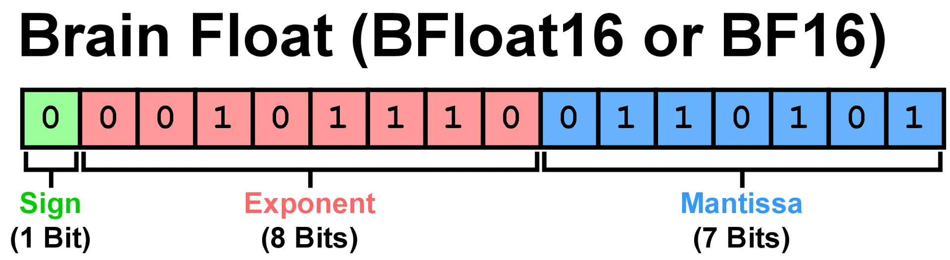
BFloat16 (Wikipedia contributors, 2025) has become the de facto standard for modern LLMs and diffusion models (Kalamkar et al., 2019; Qi et al., 2025; Wang & Kanwar, 2019). This 16-bit floating-point format allocates its bits as follows:

1 bit for the sign (positive or negative)
8 bits for the exponent (the scale or magnitude)
7 bits for the mantissa (the precision or significant digits)

The value of a BFloat16 number is calculated as:

\text{value} = (-1)^{\text{sign}} \times 2^{\text{exponent} - 127} \times (1.\text{mantissa})

This format is popular because it balances two competing needs. Compared to FP32 (the full 32-bit float), it uses half the memory. Compared to FP16 (Half-precision floating-point format), it has a much wider range of values it can represent because it dedicates more bits to the exponent (Wikipedia contributors, 2025b, 2025a). This wider range matters during training, where we need to avoid overflow and underflow (Google Cloud, 2019; Kalamkar et al., 2019).

Here's what the bit allocation looks like:

BFloat16 Structure

Shannon Entropy: Measuring Information Content

To understand why bfloat16 is wasteful, let's first examine Shannon entropy: a concept that is more intuitive than it might initially appear.

Shannon entropy measures the actual information content in data. It answers a fundamental question: "How many bits are truly needed to represent this information optimally?" (Shannon, 1948)

The formula looks like this:

H(X) = -\sum_{x} p(x) \log_2 p(x)

where $p(x)$ is the probability of seeing value $x$ .

Suppose we're encoding messages where:

"A" appears 50% of the time
"B" appears 25% of the time
"C" appears 25% of the time

The entropy is:

H = -(0.5 \log_2 0.5 + 0.25 \log_2 0.25 + 0.25 \log_2 0.25) = 1.5 \text{ bits}

This means we could encode these messages with an average of 1.5 bits per symbol using variable-length codes, even though naively assigning 2 bits to each of the 3 symbols would use more space than necessary.

The key insight: if all three symbols appeared equally (33.3% each), the entropy would be:

H = -3 \times (0.333 \log_2 0.333) \approx 1.58 \text{ bits}

When distributions are more uniform, more bits are needed. When concentrated on a few values, fewer bits suffice. Entropy quantifies this relationship.

When a field has $n$ bits, it can represent up to $2^n$ different values. If all those values appeared with equal probability, the entropy would be exactly $n$ bits. However, if most values never appear, or if a few values dominate, the entropy drops—sometimes dramatically.

The Exponent Entropy Experiment

To investigate this phenomenon, (Zhang et al., 2025) analyzed a comprehensive set of modern LLMs—Llama 3.1, Qwen 2.5, Mistral, Gemma, and others—measuring the Shannon entropy of each component of their BFloat16 weights.

The analysis examined all linear projection matrices (the main weight matrices in transformers) and computed the entropy separately for:

The sign bit
The 8 exponent bits
The 7 mantissa bits

Entropy Analysis

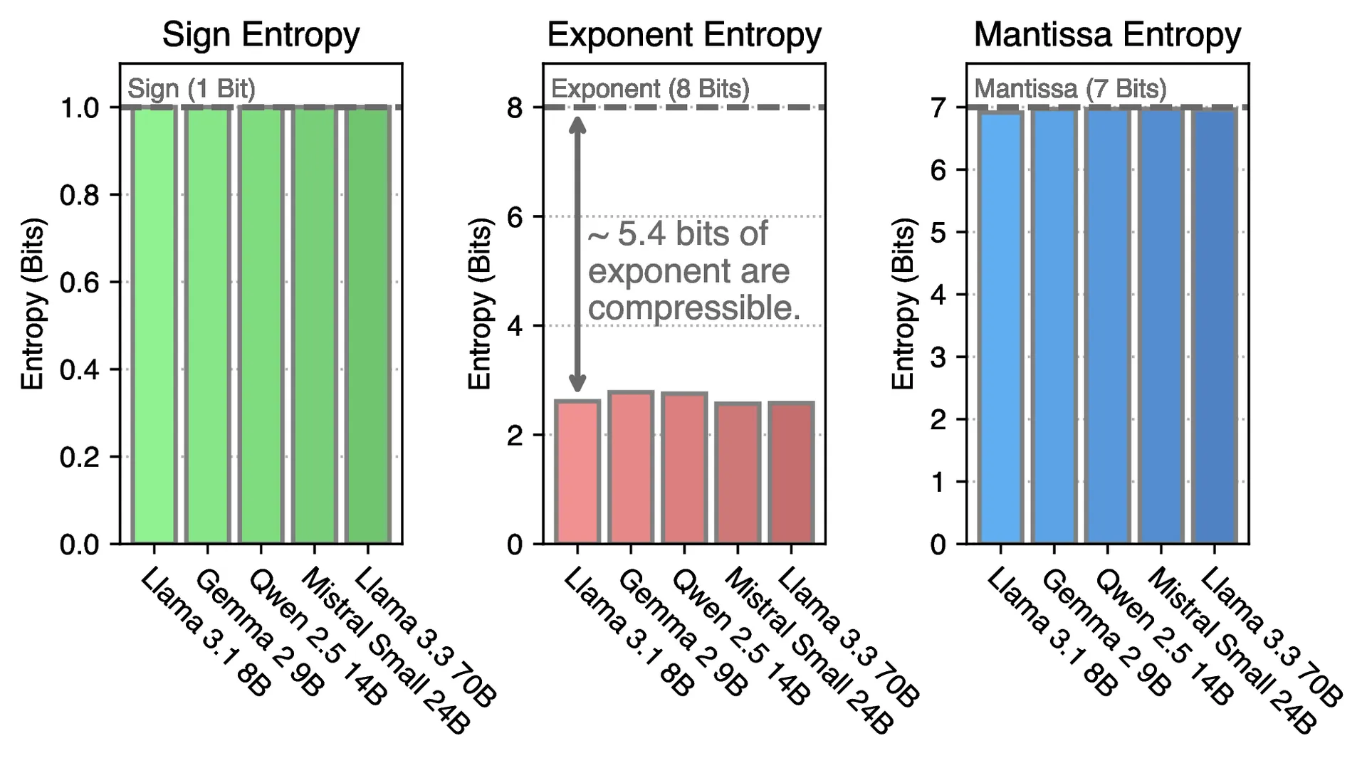
Look at that middle panel (exponent entropy). Across every model, the exponent entropy hovers around 2.6 bits. Not 8 bits. Not even 4 bits. About 2.6 bits.

Meanwhile, the sign bit has entropy close to 1 bit (makes sense—it's fairly balanced between positive and negative), and the mantissa has entropy close to 7 bits (also expected—those bits are well-utilized for precision).

Why Are Exponents So Predictable?

To understand why the exponent field is so wasteful, consider that the exponent can theoretically take any of 256 values (from 0 to 255 in the 8-bit representation). If all 256 values appeared with equal frequency, the entropy would be exactly 8 bits.

However, the actual distribution of exponent values in trained LLM weights reveals two striking patterns:

Pattern 1: Most Values Never Appear

Out of 256 possible exponent values, only about 40 are ever used. The remaining 216 values simply never appear in the weights, representing a massive allocation of unused representation capacity.

Pattern 2: The Distribution Is Extremely Skewed

Among those ~40 values that do appear, the distribution is wildly imbalanced. A handful of exponent values are extremely common, and the rest are rare.

This is what statisticians call a Zipfian or power-law distribution (Wikipedia contributors, 2025c). When exponents are ranked by frequency and plotted, the curve drops off steeply. The most common exponent might appear in 20% of all weights, the second most common in 12%, the third in 8%, and so on, declining rapidly toward zero.

This highly skewed distribution is precisely the scenario where entropy is much lower than the allocated bit-width. A few frequent values dominate, while the majority of the representation space remains unutilized.

Why Does This Happen?

The question naturally arises: why do trained neural networks produce such a skewed distribution of exponents?

The explanation relates to how neural networks learn and the characteristics their weights exhibit after training. During training, weights settle into ranges that are effective for the task. Some layers require large weights (high exponents), others require small weights (low exponents), but within a layer, weights often cluster around similar magnitudes (Xiao et al., 2023).

Moreover, techniques like weight initialization, normalization (LayerNorm, BatchNorm), and regularization all push weights toward certain ranges (Kalamkar et al., 2019). The result is that even though BFloat16 can represent values from $10^{-38}$ to $10^{38}$ , the weights in a trained model occupy a much narrower range (Google Cloud, 2019; Wikipedia contributors, 2025a).

BFloat16 is designed to handle any floating-point computation during training. However, once training is complete, the weights have converged to a much narrower range of values. The exponent field is over-provisioned for its actual usage pattern (Heilper & Singer, 2025; Kalamkar et al., 2019).

The Entropy Is Consistent Across Models

One of the most interesting findings is the remarkable consistency of this pattern. Across diverse scenarios:

1.5B parameter models vs. 70B parameter models
Llama vs. Qwen vs. Mistral vs. Gemma
Instruction-tuned models vs. base models
Reasoning models vs. standard LLMs

The exponent entropy consistently remains in the range of 2.5 to 2.7 bits.

What About Sign and Mantissa?

For completeness, let's examine the other components:

Sign bit: The entropy is close to 1 bit, which is expected. In a neural network, roughly half the weights are positive and half are negative (especially after bias subtraction or zero-centering). The sign bit efficiently carries close to 1 bit of information.

Mantissa: The entropy approaches 7 bits, which is also expected. The mantissa encodes the precision of the number—the significant digits. These must be varied and unpredictable to capture the nuances of learned representations. If the mantissa were highly compressible, it would indicate coarse weight granularity, which would degrade performance. A mantissa entropy near 7 bits is precisely what we should observe.

The exponent is the outlier—the only component dramatically underutilizing its allocated space.

Quantifying the Waste

To put this in perspective, consider the utilization of a BFloat16 number:

1 bit for sign (entropy ≈ 1 bit) → 100% utilization
8 bits for exponent (entropy ≈ 2.6 bits) → 32.5% utilization
7 bits for mantissa (entropy ≈ 7 bits) → 100% utilization

Overall, out of 16 bits, only about 10.6 bits carry actual information. The exponent alone wastes more than 5 bits per number.

Now multiply that by billions of parameters. For a model like Llama 3.1 8B (8 billion parameters), that's:

8 \times 10^9 \text{ parameters} \times 5 \text{ wasted bits per parameter} = 40 \text{ billion wasted bits} = 5 \text{ GB of wasted space}

And for Llama 3.1 405B, we're talking about hundreds of gigabytes of wasted storage, just from the exponent inefficiency.

Opportunities for Compression

This inefficiency presents a significant opportunity. If the exponent has entropy around 2.6 bits but requires 8 bits to store, substantial compression is possible.

The crucial qualifier is lossless compression. Rather than approximating weights or discarding information (as quantization does), we can exploit the statistical redundancy in exponent distributions to store the exact same information in less space.

One way to do this is with entropy coding techniques like Huffman coding (Huffman, 1952). The idea is simple:

Assign short codes to frequent exponent values
Assign longer codes to rare exponent values
Pack everything tightly at the bit level

Because frequent values receive short codes, the average code length approaches the entropy (2.6 bits)—near-optimal compression.

For the sign and mantissa, which are already efficiently utilized, no compression is applied. However, the exponent can be compressed from 8 bits down to approximately 2.6 bits on average (Zhang et al., 2025).

The result is a floating-point format that uses about 11 bits instead of 16 bits—a 30% reduction—while preserving every bit of the original information (Zhang et al., 2025). Decompression recovers the exact original BFloat16 numbers with zero loss.

Practical Implications

The question arises: why does saving 5 bits per number matter?

Several significant benefits emerge:

1. Memory constraints. GPU memory represents the primary bottleneck for running large LLMs. A model like Llama 3.1 405B requires 810 GB in BFloat16, exceeding the capacity of a single GPU node with 8×80GB cards. Compressing to 70% of the original size enables deployment on a single node, effectively halving hardware requirements.

2. Extended context lengths. During inference, the KV cache grows linearly with generated tokens. When model weights consume less memory, more capacity remains available for the KV cache, enabling longer sequence generation before memory exhaustion.

3. Genuine losslessness. Unlike quantization (which approximates weights), entropy-based compression preserves original values exactly. This is critical for applications requiring bit-exact behavior—regulated industries, scientific computing, or production deployments that must match validated models.

4. Composability. Lossless compression can be combined with other memory-saving techniques without compounding errors. For instance, one can quantize the KV cache while maintaining exact weight precision.

What is next?

In the next post, we'll see how entropy evolves during training, and how different initialization and training recipes affect the exponent distribution.

Google Cloud. (2019). Improve Your Model’s Performance with bfloat16. https://cloud.google.com/tpu/docs/bfloat16

Heilper, A., & Singer, D. (2025). Lossless Compression of Neural Network Components: Weights, Checkpoints, and K/V Caches in Low-Precision Formats. arXiv Preprint. https://arxiv.org/abs/2508.19263

Huffman, D. A. (1952). A Method for the Construction of Minimum-Redundancy Codes. Proceedings of the IRE, 40(9), 1098–1101. https://doi.org/10.1109/JRPROC.1952.273898

Kalamkar, D., Mudigere, D., Mellempudi, N., Das, D., Banerjee, K., Avancha, S., Vooturi, D. T., Jammalamadaka, N., Huang, J., Yuen, H., Yang, J., Park, J., Heinecke, A., Georganas, E., Srinivasan, S., Kundu, A., Smelyanskiy, M., Kaul, B., & Dubey, P. (2019). A Study of BFLOAT16 for Deep Learning Training. arXiv Preprint. https://arxiv.org/abs/1905.12322

Qi, P., Liu, Z., Zhou, X., Pang, T., Du, C., Lee, W. S., & Lin, M. (2025). Defeating the Training-Inference Mismatch via FP16. arXiv Preprint arXiv:2510.26788.

Shannon, C. E. (1948). A Mathematical Theory of Communication. Bell System Technical Journal, 27(3), 379–423. https://doi.org/10.1002/j.1538-7305.1948.tb01338.x

Wang, S., & Kanwar, P. (2019). BFloat16: The Secret to High Performance on Cloud TPUs. https://cloud.google.com/blog/products/ai-machine-learning/bfloat16-the-secret-to-high-performance-on-cloud-tpus

Wikipedia contributors. (2025a). Bfloat16 floating-point format. https://en.wikipedia.org/wiki/Bfloat16_floating-point_format

Wikipedia contributors. (2025b). Half-precision floating-point format. https://en.wikipedia.org/wiki/Half-precision_floating-point_format

Wikipedia contributors. (2025c). Zipf’s law. https://en.wikipedia.org/wiki/Zipf%27s_law

Xiao, X., Li, Z., Xie, C., & Zhou, F. (2023). Heavy-Tailed Regularization of Weight Matrices in Deep Neural Networks. Artificial Neural Networks and Machine Learning – ICANN 2023, 236–247. https://doi.org/10.1007/978-3-031-44204-9_20

Zhang, T., Hariri, M., Zhong, S., Chaudhary, V., Sui, Y., Hu, X., & Shrivastava, A. (2025). 70% Size, 100% Accuracy: Lossless LLM Compression for Efficient GPU Inference via Dynamic-Length Float (DFloat11). The Thirty-Ninth Annual Conference on Neural Information Processing Systems. https://arxiv.org/pdf/2504.11651