Entropy of bfloat16 During Training: How Optimizers Shape Weight Distributions
TL;DR: Trained LLMs consistently show ~2.6 bits of exponent entropy. We trained neural networks to understand how this emerges. Surprising discovery: the optimizer matters more than initialization. AdamW consistently produces distributions near 2.6 bits regardless of how weights are initialized, explaining why LLMs (which typically use AdamW) show such consistent entropy patterns.
The 2.6 Bits Mystery
In the previous post, we discussed that trained LLMs waste significant space in their BFloat16 representations (Zhang et al., 2025). While the exponent field has 8 bits available (theoretically representing 256 different values), it carries only about 2.6 bits of actual information.
This finding was remarkably consistent across models:
- Small (1.5B) to large (70B) parameter counts
- Different architectures (Llama, Qwen, Mistral, Gemma)
- Various training objectives (base models, instruction-tuned, reasoning)
All showed exponent entropy hovering around 2.5 to 2.7 bits.
This consistency raised a natural question: How does training produce this specific value?
The Experiment
To understand how exponent entropy evolves during training, we conducted a systematic study:
We trained neural networks from scratch, tracking the distribution of sign, exponent, and mantissa bits at regular intervals throughout training. We tested multiple combinations:
Initializations: Xavier (Glorot & Bengio, 2010), Kaiming (He et al., 2015), Orthogonal, Normal, Uniform
Optimizers: SGD (Sutskever et al., 2013), Adam (Kingma & Ba, 2015), AdamW (Loshchilov & Hutter, 2019)
Total: 15 different configurations
Each model was trained for 50 epochs while we measured the entropy of all three BFloat16 components every 5 epochs.
What Trained Weights Look Like
Before examining how distributions evolve, let's look at what a trained model's weight distribution looks like.

This figure shows the distribution of sign, exponent, and mantissa values in a trained neural network (Kalamkar et al., 2019). Each bar represents how frequently that particular bit pattern appears in the model's weights.
Sign (left panel): The distribution is nearly balanced—roughly half the weights are positive, half negative. This gives entropy close to 1 bit, meaning the sign bit is fully utilized.
Mantissa (right panel): The distribution appears fairly uniform across the 128 possible values (0-127) (Wikipedia contributors, 2025). The entropy approaches 7 bits, indicating that precision bits are well-utilized to capture fine-grained weight variations.
Exponent (middle panel): This is where things get interesting. Despite having 256 possible values (0-255), the distribution is highly peaked. Only about 40-50 exponent values ever appear, and among those, a few dominate. The rest of the representation space sits unused.
This concentrated distribution is exactly what produces the low entropy of ~2.6 bits we observed in trained LLMs.
The Evolution During Training
Now let's examine how these distributions evolve as training progresses.
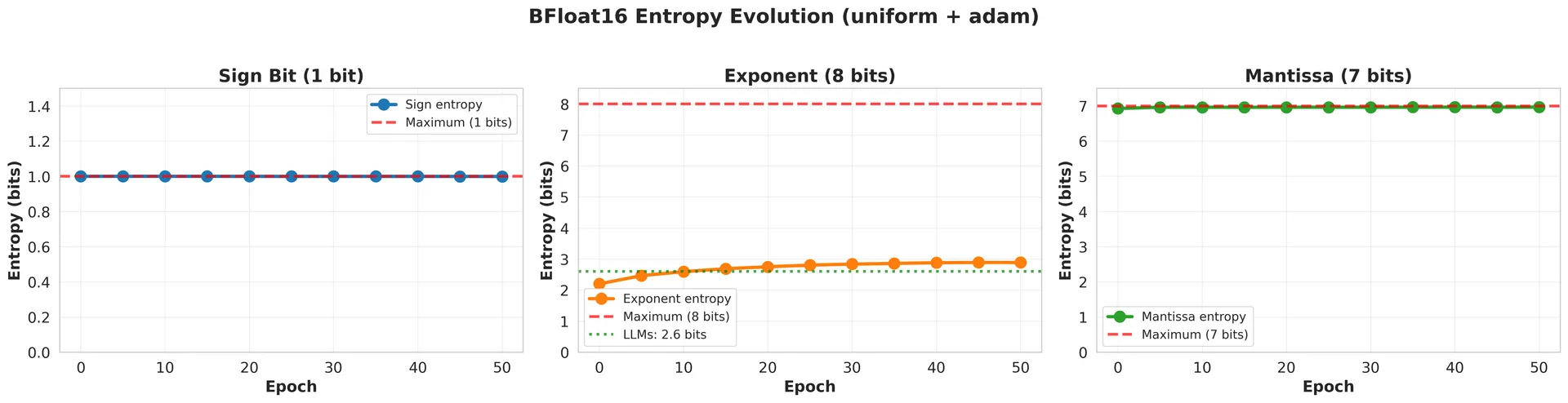
This figure tracks the entropy of all three components over 50 epochs of training:
Sign entropy (left): Starts at 1.0 bit and remains there throughout training. The balance between positive and negative weights is established immediately and stays constant.
Mantissa entropy (right): Starts near 7 bits and stays there. The precision bits remain fully utilized from initialization through convergence.
Exponent entropy (middle): This is where the action happens. It starts around 2.5 bits (already much lower than the 8 bits allocated) and changes during training—but not always in the same direction.
The green dashed line marks 2.6 bits, the value consistently observed in trained LLMs. Notice that the exponent entropy fluctuates around this value but doesn't necessarily converge to it.
The Role of Optimizers
We expected that initialization methods would determine the final entropy. Instead, we discovered that the optimizer shapes the weight distribution far more than initialization does.
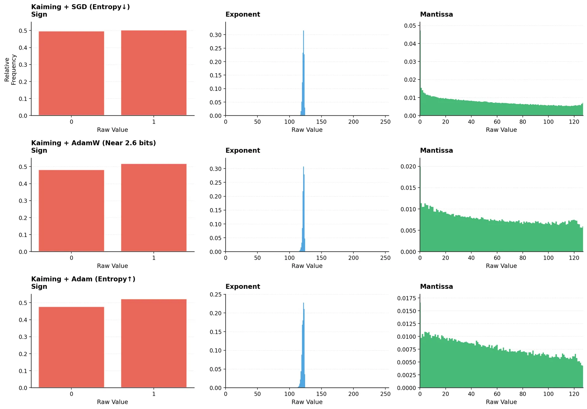
This figure shows three models with identical initialization (Kaiming) but different optimizers. Look at the exponent panels (middle column):
SGD (top row): The distribution becomes highly concentrated. Exponents cluster tightly around a few values, producing very low entropy (around 2.4 bits). The compression of the distribution is dramatic.
AdamW (middle row): The distribution shows moderate spread. The peak is less pronounced than SGD, and the entropy sits near 2.6 bits—matching what we see in trained LLMs.
Adam (bottom row): The distribution is more spread out. More exponent values appear with meaningful frequency, pushing entropy toward 2.9 bits.
Same initialization, three completely different outcomes. The optimizer isn't just affecting how fast the model converges, it's fundamentally changing the structure of the learned weights.
Why Optimizers Matter
The relationship between optimizers and entropy becomes clearer when we examine the mechanisms:
SGD with momentum (Sutskever et al., 2013) updates all weights proportionally to their gradients. This tends to push weights toward smaller magnitudes over time, concentrating the exponent distribution.
Adam (Kingma & Ba, 2015) maintains per-parameter adaptive learning rates. These adaptive updates allow different parameters to explore different ranges of values, leading to a broader distribution of exponents and higher entropy.
AdamW (Loshchilov & Hutter, 2019) combines Adam's adaptive learning rates with decoupled weight decay. The weight decay term explicitly pushes weights toward zero, but the adaptive learning rates allow parameters to resist this pull when gradients are strong. This balance produces distributions with moderate spread—neither as concentrated as SGD nor as spread out as Adam.
The AdamW Consistency
The most interesting observation emerges when we look at AdamW across different initializations:
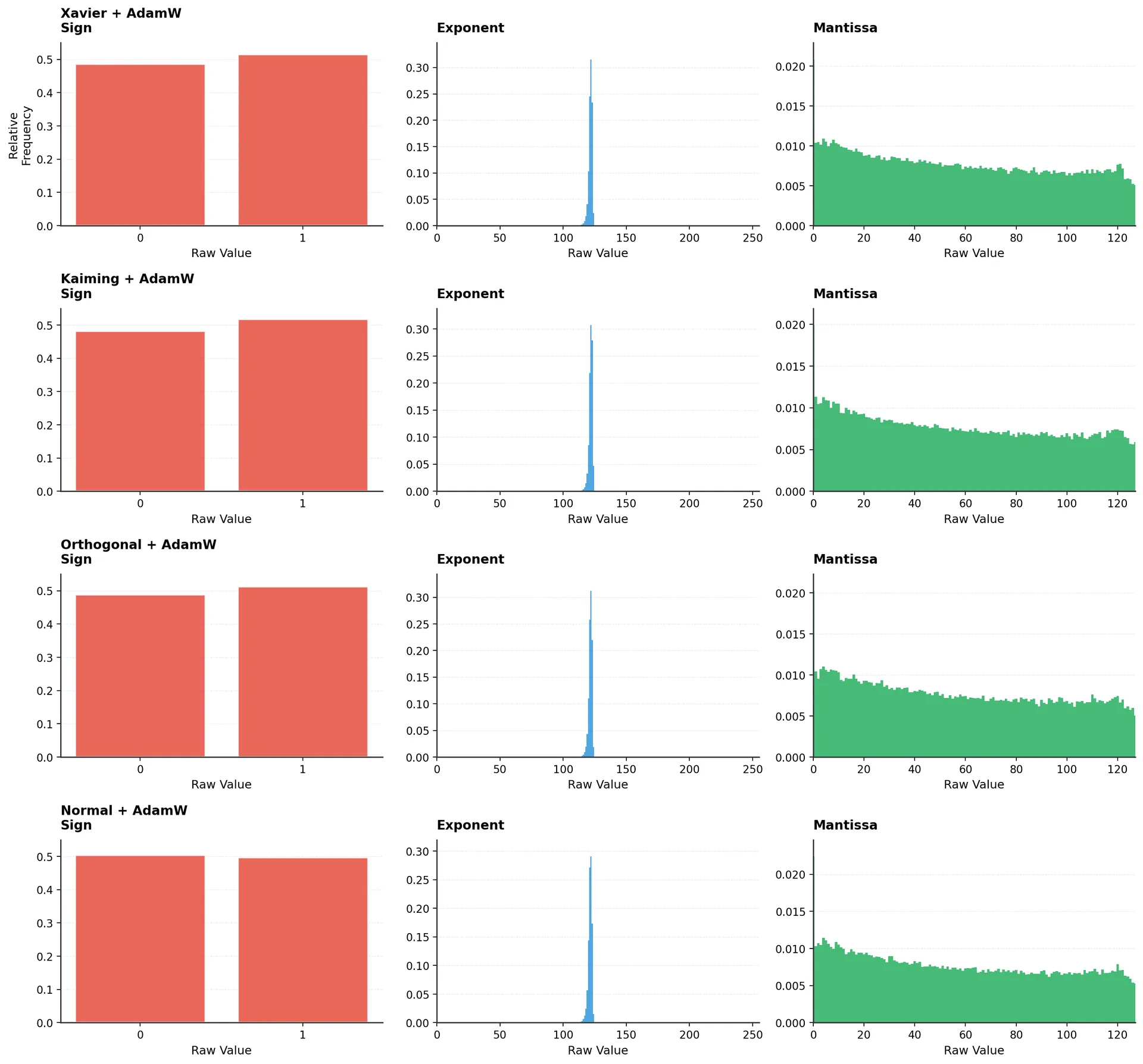
Four different initializations (Xavier, Kaiming, Orthogonal, Normal), all trained with AdamW. Look at the exponent distributions (middle column).
Despite starting from different initial configurations, all four models converge to remarkably similar exponent distributions. The shapes of the distributions are nearly identical, and all produce entropy around 2.4-2.5 bits.
This consistency is striking because:
- Xavier (Glorot & Bengio, 2010) and Kaiming (He et al., 2015) use different scaling strategies
- Orthogonal starts with structured, non-random weights
- Normal uses a simple Gaussian distribution
Yet AdamW's training dynamics override these initial differences, producing consistent final distributions.
Why LLMs Show 2.6 Bits
This brings us to the answer to our original question: why do trained LLMs consistently show exponent entropy around 2.6 bits?
The answer isn't primarily about scale, architecture, or training data. It's simpler: modern LLMs are trained with AdamW.
Our observations show that AdamW naturally produces exponent distributions with entropy in the 2.4-2.6 bit range, regardless of initialization. This happens because:
Weight decay constrains magnitude ranges: The explicit weight decay in AdamW prevents weights from growing too large, limiting the range of exponents needed.
Adaptive learning rates preserve structure: Unlike pure weight decay (as in SGD with L2 regularization), AdamW's adaptive rates allow important parameters to maintain larger magnitudes when needed, preventing over-compression of the distribution.
Independence from initialization: The optimizer's dynamics are strong enough that initial weight distributions matter less than how weights are updated during training.
When training large language models, practitioners consistently choose AdamW because it works well for the task. A side effect of this choice is that the resulting models all exhibit similar weight distributions—and thus similar entropy patterns.
Comparison Across All Experiments
To see the full picture, let's look at how exponent entropy evolved across all 15 experiments:
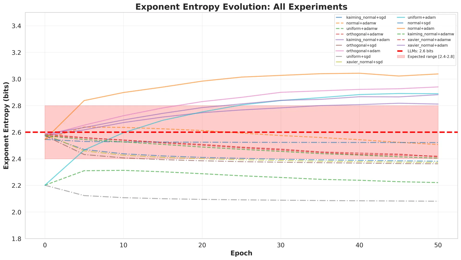
Each line represents one combination of initialization and optimizer. The red dashed line marks 2.6 bits, and the shaded region shows the [2.4, 2.8] range observed in trained LLMs.
Several patterns emerge:
Divergence, not convergence: Rather than all experiments converging to a single value, we see divergent paths. Some decrease entropy (moving toward more compressible weights), others increase it.
Optimizer clustering: Lines group by optimizer more than by initialization. The SGD lines (dash-dot) trend lower, Adam lines (solid) trend higher, and AdamW lines (dashed) cluster near 2.6 bits.
Limited convergence to LLM range: Only about one-third of experiments land in the [2.4, 2.8] range. Notably, most of these are AdamW experiments.
From Initialization to Trained State
The transition from initial to final entropy reveals the optimizer's influence:
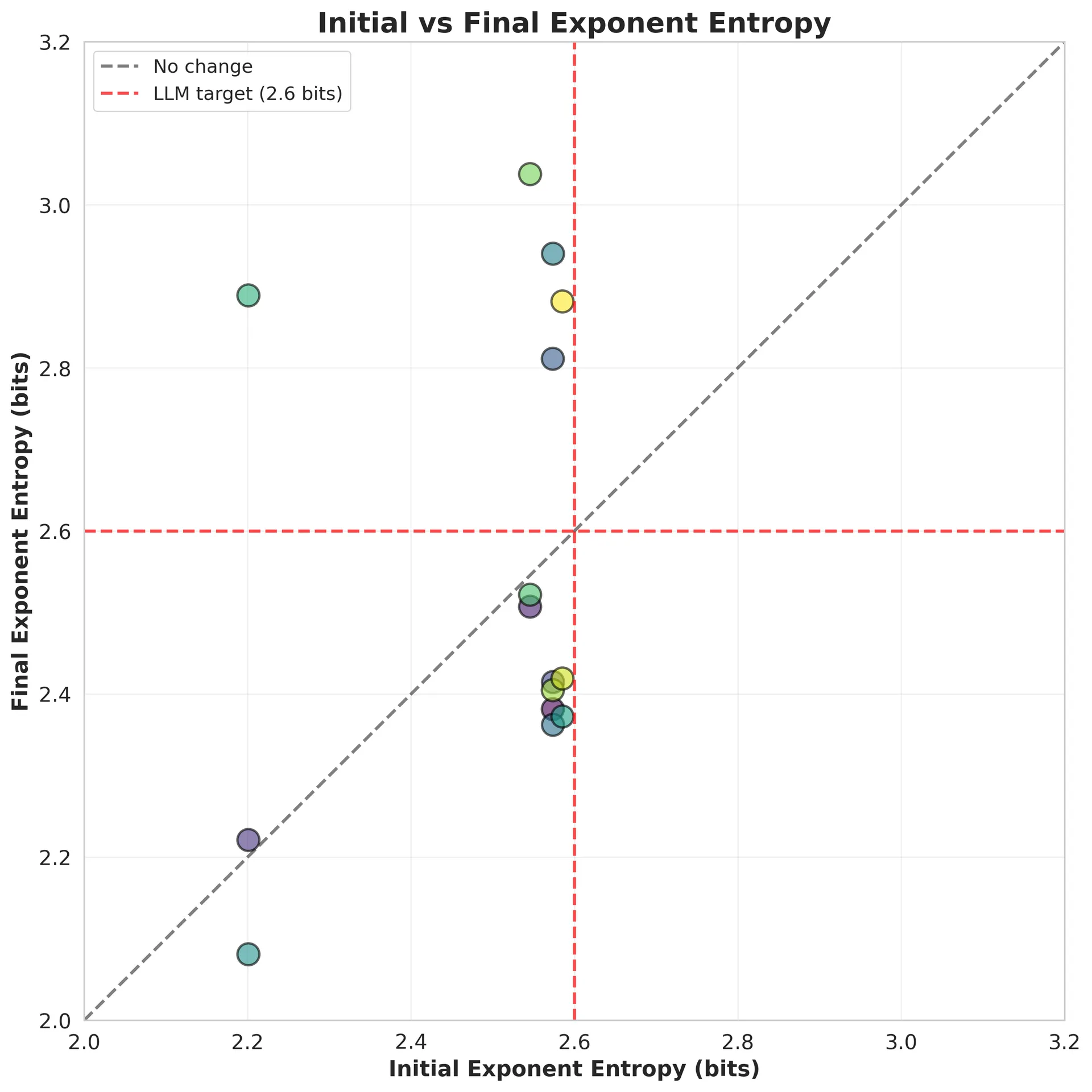
Each point represents one experiment. The x-axis shows initial entropy (right after initialization), the y-axis shows final entropy (after 50 epochs). The diagonal line represents "no change."
Points above the diagonal increased entropy during training. Points below decreased entropy. The red lines mark the 2.6 bits target.
Most experiments change: Very few points sit on the diagonal. Training actively reshapes weight distributions.
Predictable by optimizer: Points don't cluster by initialization method, but they do cluster by optimizer. Adam experiments (not shown separately) tend to sit above the diagonal. SGD experiments below. AdamW experiments near the target.
Initial state matters less: Points start at different x-coordinates (different initial entropies) but end up grouped by optimizer (y-coordinate). The journey's destination depends more on the path taken (optimizer) than the starting point (initialization).
What About Sign and Mantissa?
Throughout all our experiments, sign and mantissa behaved predictably:
Sign entropy remained at 1.0 bit across all configurations and throughout training. The balance between positive and negative weights is established immediately and maintained.
Mantissa entropy stayed near 7.0 bits. These precision bits remain fully utilized regardless of optimizer or initialization. This makes sense: the mantissa encodes fine-grained weight values, and any compression here would directly hurt model expressiveness.
Exponent entropy showed high variability (2.1 to 3.0 bits across experiments) and optimizer-dependent evolution. This is the only component where training dynamics significantly reshape the distribution.
The exponent's behavior differs because it encodes weight magnitude rather than precision (Xiao et al., 2023). Optimizers directly influence magnitude through their update rules and regularization strategies, but precision requirements remain constant.
Implications for Model Compression
These findings have practical implications for model compression:
Optimizer choice affects compressibility: Models trained with different optimizers have different compression potential (Zhang et al., 2025). AdamW models achieve ~32% exponent field utilization (2.6 / 8 bits), while SGD models can reach ~27% (2.1 / 8 bits), and Adam models show ~36% (2.9 / 8 bits).
For a model with 7 billion parameters, this difference translates to:
- AdamW: ~5.5 GB for exponents
- SGD: ~4.7 GB for exponents
- Adam: ~6.3 GB for exponents
That's a potential 1.6 GB difference in compressed size, purely from optimizer choice.
Initialization matters less than expected: While different initializations produce different initial entropy values, the optimizer's training dynamics dominate the final outcome. This suggests that compression-aware training should focus on optimizer selection rather than initialization schemes.
Training dynamics are predictable: The relationship between optimizer and final entropy is consistent enough to be useful. When deploying models, we can predict their compression potential based on knowing which optimizer was used during training.
What is next?
In the next post, we'll see how to put these insights into action using common LLM inference tools like vLLM and Hugging Face Transformers.
Comments